JPEG XL and the Pareto Front

Version 0.10 of libjxl, the reference implementation for JPEG XL, has just been released. The main improvement this version brings, is that the so-called “streaming encoding” API has now been fully implemented. This API allows encoding a large image in “chunks.” Instead of processing the entire image at once, which may require a significant amount of RAM if the image is large, the image can now be processed in a more memory-friendly way. As a side effect, encoding also becomes faster, in particular when doing lossless compression of larger images.

Before version 0.10, lossless JPEG XL encoding was rather memory-intensive and could take quite some time. This could pose a serious problem when trying to encode large images, like for example this 13500×6750 NASA image of Earth at night (64 MB as a TIFF file, 273 MB uncompressed).

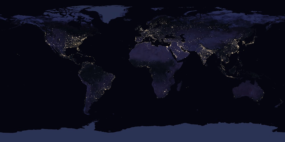
Compressing this image required about 8 gigabytes of RAM in libjxl version 0.9, at the default effort (e7). It took over two minutes, and resulted in a jxl file of 33.7 MB, which is just under 3 bits per pixel. Using more threads did not help much: using a single thread it took 2m40s, using eight threads that was reduced to 2m06s. These timings were measured on a November 2023 Macbook Pro with a 12-core Apple M3 Pro CPU with 36 GB of RAM.

Upgrading to libjxl version 0.10, compressing this same image now requires only 0.7 gigabytes of RAM, takes 30 seconds using a single thread (or 5 seconds using eight threads), and results in a jxl file of 33.2 MB.

For other effort settings, these are the results for this particular image:

effort setting	memory 0.9.2	memory 0.10	time 0.9	time 0.10	compressed size 0.9	compressed size 0.10	memory reduction	speedup
e1, 1 thread	821 MB	289 MB	0.65s	0.3s	65.26 MB	67.03 MB	2.8x	2.2x
e1, 8 threads	842 MB	284 MB	0.21s	0.1s	65.26 MB	67.03 MB	2.9x	2.1x
e2, 1 thread	7,503 MB	786 MB	4.3s	3.6s	49.98 MB	44.78 MB	9.5x	1.2x
e2, 8 threads	6,657 MB	658 MB	2.2s	0.7s	49.98 MB	44.78 MB	10.1x	3.0x
e3, 8 threads	7,452 MB	708 MB	2.4s	1.3s	45.20 MB	44.23 MB	10.5x	1.8x
e7, 1 thread	9,361 MB	748 MB	2m40s	30s	33.77 MB	33.22 MB	12.5x	4.6x
e7, 8 threads	7,887 MB	648 MB	2m06s	5.4s	33.77 MB	33.22 MB	12.2x	23.6x
e8, 8 threads	9,288 MB	789 MB	7m38s	22.2s	32.98 MB	32.93 MB	11.8x	20.6x
e9, 8 threads	9,438 MB	858 MB	21m58s	1m46s	32.45 MB	32.20 MB	11.0x	12.4x

As you can see in the table above, compression is a game of diminishing returns: as you increase the amount of cpu time spent on the encoding, the compression improves, but not in a linear fashion. Spending one second instead of a tenth of a second (e2 instead of e1) can in this case shave off 22 megabytes; spending five seconds instead of one (e7 instead of e2) shaves off another 11 megabytes. But to shave off one more megabyte, you’ll have to wait almost two minutes (e9 instead of e7).

So it’s very much a matter of trade-offs, and it depends on the use case what makes the most sense. In an authoring workflow, when you’re saving an image locally while still editing it, you typically don’t need strong compression and low-effort encoding makes sense. But in a one-to-many delivery scenario, or for long-term archival, it may well be worth it to spend a significant amount of CPU time to shave off some more megabytes.

When comparing different compression techniques, it doesn’t suffice to only look at the compressed file sizes. The speed of encoding also matters. So there are two dimensions to consider: compression density and encode speed.

A specific method can be called Pareto-optimal if no other method can achieve the same (or better) compression density in less time. There might be other methods that compress better but take more time, or that compress faster but result in larger files. But a Pareto-optimal method delivers the smallest files for a given time budget, which is why it’s called “optimal.”

The set of Pareto-optimal methods is called the “Pareto front.” It can be visualized by putting the different methods on a chart that shows both dimensions — encode speed and compression density. Instead of looking at a single image, which may not be representative, we look at a set of images and look at the average speed and compression density for each encoder and effort setting. For example, for this set of test images, the chart looks like this:

The vertical axis shows the encode speed, in megapixels per second. It’s a logarithmic scale since it has to cover a broad range of speeds, from less than one megapixel per second to hundreds of megapixels per second. The horizontal axis shows the average bits per pixel for the compressed image (uncompressed 8-bit RGB is 24 bits per pixel).

For AVIF, the darker points indicate a faster but slightly less dense tiled encoder setting (using –tilerowslog2 2 –tilecolslog2 2), which is faster because it can make better use of multi-threading, while the lighter points indicate the default non-tiled setting. For PNG, the result of libpng with default settings is shown here as a reference point; other PNG encoders and optimizers exist that reach different trade-offs.

The previous version of libjxl already achieved Pareto-optimal results across all speeds, producing smaller files than PNG and lossless AVIF or lossless WebP. The new version beats the previous version by a significant margin.

Not shown on the chart is QOI, which clocked in at 154 Mpx/s to achieve 17 bpp, which may be “quite OK” but is quite far from Pareto-optimal, considering the lowest effort setting of libjxl compresses down to 11.5 bpp at 427 Mpx/s (so it is 2.7 times as fast and the result is 32.5% smaller).

Of course in these charts, quite a lot depends on the selection of test images. In the chart above, most images are photographs, which tend to be hard to compress losslessly: the naturally occurring noise in such images is inherently incompressible.

For non-photographic images, things are somewhat different. I took a random collection of manga images in various drawing styles (41 images with an average size of 7.3 megapixels) and these were the results:

These kinds of images compress significantly better, to around 4 bpp (compared to around 10 bpp for photographic images). For these images, lossless AVIF is not useful — it compresses worse than PNG, and reaches about the same density as QOI but is much slower. Lossless WebP on the other hand achieves very good compression for such images. For these types of images, QOI is indeed quite OK for its speed (and simplicity), though far from Pareto-optimal: low-effort JPEG XL encoding is twice as fast and 31% smaller.

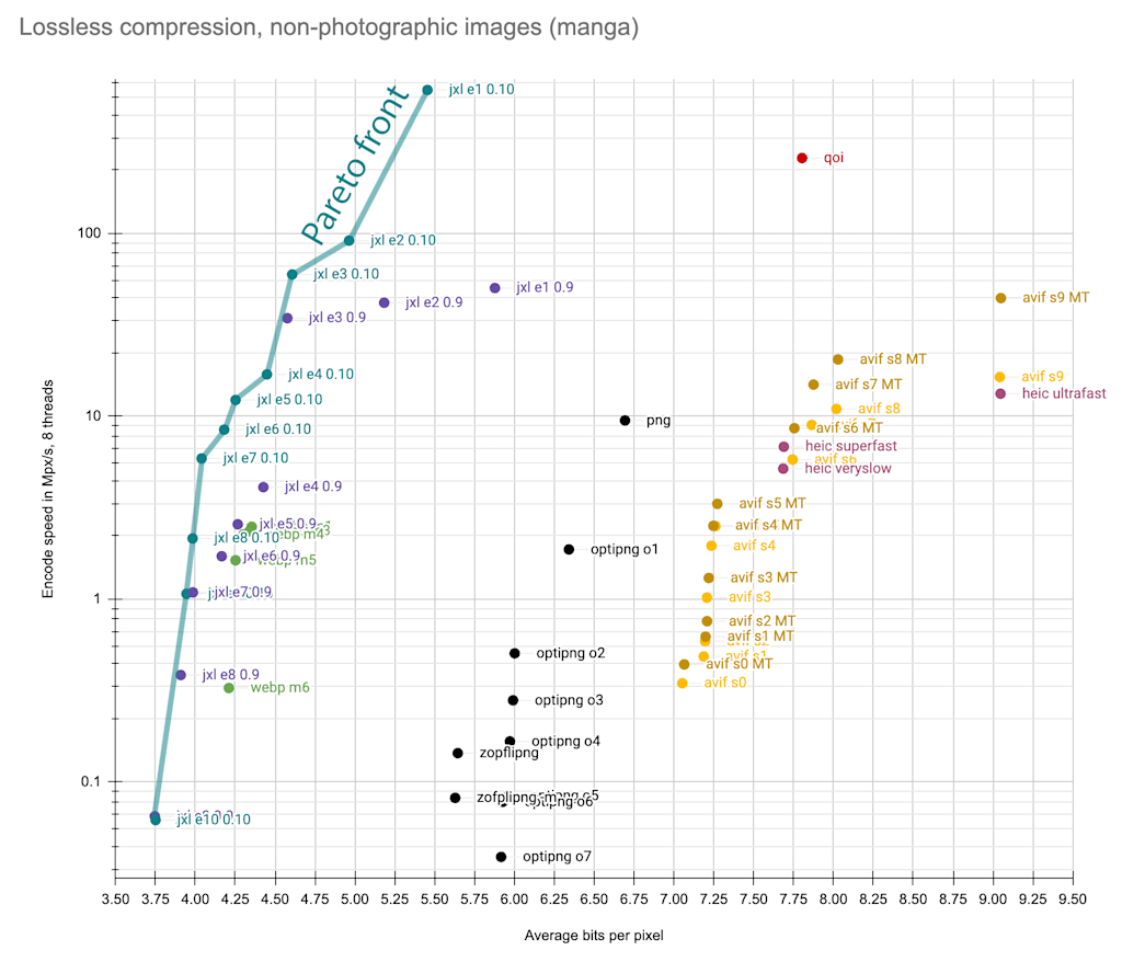
For non-photographic images, the new version of libjxl again improves upon the previous version, by a significant margin. The previous version of libjxl could just barely beat WebP: e.g. default-effort WebP compressed these images to 4.30 bpp at 2.3 Mpx/s, while libjxl 0.9 at effort 5 compressed them to 4.27 bpp at 2.6 Mpx/s — only a slight improvement. However libjxl 0.10 at effort 5 compresses the images to 4.25 bpp at 12.2 Mpx/s (slightly better compression but much faster), and at effort 7 it compresses them to 4.04 bpp at 5.9 Mpx/s (significantly better compression and still twice as fast). Zooming in on the medium-speed part of the Pareto front on the above plot, the improvement going from libjxl 0.9 to 0.10 becomes clear:

Lossless compression is relatively easy to benchmark: all that matters is the compressed size and the speed. For lossy compression, there is a third dimension: image quality.

Lossy image codecs and encoders can perform differently at different quality points. An encoder that works very well for high-quality encoding does not necessarily also perform well for low-quality encoding, and the other way around.

Of these three dimensions (compression, speed and quality), often speed is simply ignored, and plots are made of compression versus quality (also known as bitrate-distortion plots). But this does not really allow evaluating the trade-offs between encode effort (speed) and compression performance. So if we really want to investigate the Pareto front for lossy compression, one way of doing it is to look at different “slices” of the three-dimensional space, at various quality points.

Image quality is a notoriously difficult thing to measure: in the end, it is subjective and somewhat different from one human to the next. The best way to measure image quality is still to run an experiment involving at least dozens of humans looking carefully at images and comparing or scoring them, according to rigorously defined test protocols. At Cloudinary, we have done such experiments in the past. But while this is the best way to assess image quality, it is a time-consuming and costly process, and it is not feasible to test all possible encoder configurations in this way.

For that reason, so-called objective metrics are being developed, which allow algorithmic estimates of image quality. These metrics are not “more objective” (in the sense of “more correct”) than scores obtained from testing with humans, in fact they are less “correct.” But they can give an indication of image quality much faster and cheaper (and more easily reproducible and consistent) than when humans are involved, which is what makes them useful.

The best metrics currently publicly available are SSIMULACRA2, Butteraugli, and DSSIM. These metrics try to model the human visual system and have the best correlation with subjective results. Older, simpler metrics like PSNR or SSIM could also be used, but they do not correlate very well with human opinions about image quality. Care has to be taken not to measure results using a metric an encoder is specifically optimizing for, as that would skew the results in favor of such encoders. For example, higher-effort libjxl optimizes for Butteraugli, while libavif can optimize for PSNR or SSIM. In this respect, SSIMULACRA2 is “safe” since none of the encoders tested is using it internally for optimization.

Different metrics will say different things, but there are also different ways to aggregate results across a set of images. To keep things simple, I selected encoder settings such that when using each setting on all images in the set, the average SSIMULACRA2 score was equal to (or close to) a specific value. Another method would have been to adjust the encoder settings per image so for each image the SSIMULACRA2 score is the same, or to select an encoder setting such that the worst-case SSIMULACRA2 score is equal to a specific value.
Aligning on worst-case scores is favorable for consistent encoders (encoders that reliably produce the same visual quality given fixed quality settings), while aligning on average scores is favorable for inconsistent encoders (encoders where there is more variation in visual quality when using fixed quality settings). From earlier research, we know that AVIF and WebP are more inconsistent than JPEG and HEIC, and that JPEG XL has the most consistent encoder:

Defining the quality points the way I did (using fixed settings and aligning by average metric score) is in the favor of WebP and AVIF; in practical usage you will likely want to align on worst-case metric score (or rather, worst-case actual visual quality), but I chose not to do that, in order to not favor JPEG XL.

Lossless compression offers 2:1 to 3:1 compression ratios (8 to 12 bpp) for photographic images. Lossy compression can reach much better compression ratios. It is tempting to see how lossy image codecs behave when they are pushed to their limits. Compression ratios of 50:1 or even 200:1 (0.1 to 0.5 bpp) can be obtained, at the cost of introducing compression artifacts. Here is an example of an image compressed to reach a SSIMULACRA2 score of 50, 30, and 10 using libjpeg-turbo, libjxl and libavif:

This kind of quality is interesting to look at in experiments, but in most actual usage, it is not desirable to introduce such noticeable compression artifacts. In practice, the range of qualities that is relevant corresponds to SSIMULACRA2 scores ranging from 60 (medium quality) to 90 (visually lossless). These qualities look like this:

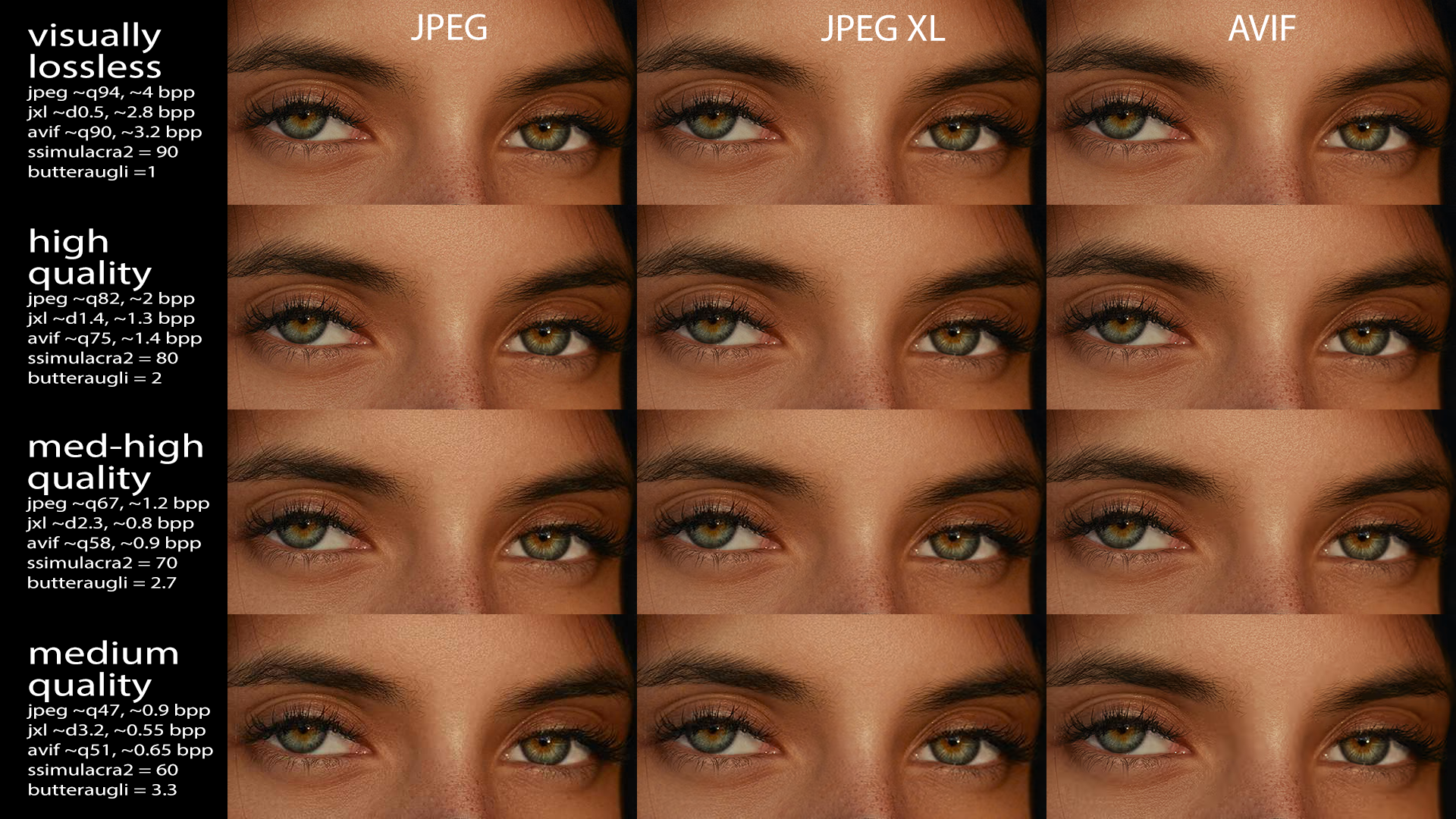
Visually lossless quality (SSIMULACRA2 = 90) can be reached with a compression ratio of about 8:1 (3 bpp) with modern codecs such as AVIF and JPEG XL, or about 6:1 (4 bpp) with JPEG. At this point, the image is visually not distinguishable from the uncompressed original, even when looking very carefully. In cameras, when not shooting RAW, typically this is the kind of quality that is desired. For web delivery, it is overkill to use such a high quality.

High quality (SSIMULACRA2 = 80) can be reached with a compression ratio of 16:1 (1.5 bpp). When looking carefully, very small differences might be visible, but essentially the image is still as good as the original. This, or perhaps something in between high quality and visually lossless quality, is the highest quality useful for web delivery, for use cases where image fidelity really matters.

Medium-high quality (SSIMULACRA2 = 70) can be reached with a compression ratio of 30:1 (0.8 bpp). There are some small artifacts, but the image still looks good. This is a good target for most web delivery use cases, as it makes a good trade-off between fidelity and bandwidth optimization.

Medium quality (SSIMULACRA2 = 60) can be reached with a compression ratio of 40:1 (0.6 bpp). Compression artifacts start to become more noticeable, but they’re not problematic for casual viewing. For non-critical images on the web, this quality can be “good enough.”

Any quality lower than this is potentially risky: sure, bandwidth will be reduced by going even further, but at the cost of potentially ruining the images. For the web, in 2024, the relevant range is medium to high quality: according to the HTTP Archive, the median AVIF image on the web is compressed to 1 bpp, which corresponds to medium-high quality, while the median JPEG image is 2.1 bpp, which corresponds to high quality. For most non-web use cases (e.g. cameras), the relevant range is high to (visually) lossless quality.

In the following Pareto front plots, the following encoders were tested:

format	encoder	version
JPEG	libjpeg-turbo	libjpeg-turbo 2.1.5.1
JPEG	sjpeg	sjpeg @ e5ab130
JPEG	mozjpeg	mozjpeg version 4.1.5 (build 20240220)
JPEG	jpegli	from libjxl v0.10.0
AVIF	libavif / libaom	libavif 1.0.3 (aom [enc/dec]:3.8.1)
JPEG XL	libjxl	libjxl v0.10.0
WebP	libwebp	libwebp 1.3.2
HEIC	libheif	heif-enc libheif version: 1.17.6 (x265 3.5)

These are the most recent versions of each encoder at the time of writing (end of February 2024).

Encode speed was again measured on a November 2023 Macbook Pro (Apple M3 Pro), using 8 threads. For AVIF, both the tiled setting (with –tilerowslog2 2 –tilecolslog2 2) and the non-tiled settings were tested. The tiled setting, indicated with “MT”, is faster since it allows better multi-threading, but it comes at a cost in compression density.

Let’s start by looking at the results for medium quality, i.e., settings that result in a corpus average SSIMULACRA2 score of 60. This is more or less the lowest quality point that is used in practice. Some images will have visible compression artifacts with these encoder settings, so this quality point is most relevant when saving bandwidth and reducing page weight is more important than image fidelity.

First of all, note that even for the same format, different encoders and different effort settings can reach quite different results. Historically, the most commonly used JPEG encoder was libjpeg-turbo — often using its default setting (no Huffman optimization, not progressive), which is the point all the way in the top right. When Google first introduced WebP, it outperformed libjpeg-turbo in terms of compression density, as can be seen in the plot above. But Mozilla was not impressed, and they created their own JPEG encoder, mozjpeg, which is slower than libjpeg-turbo but offers better compression results. And indeed, we can see that mozjpeg is actually more Pareto-efficient than WebP (for this corpus, at this quality point).

More recently, the JPEG XL team at Google has built yet another JPEG encoder, jpegli, which is both faster and better than even mozjpeg. It is based on lessons learned from guetzli and libjxl, and offers a very attractive trade-off: it is very fast, compresses better than WebP and even high-speed AVIF, while still producing good old JPEG files that are supported everywhere.

Moving on to the newer codecs, we can see that both AVIF and HEIC can obtain a better compression density than JPEG and WebP, at the cost of slower encoding. JPEG XL can reach a similar compression density but encodes significantly faster. The current Pareto front for this quality point consists of JPEG XL and the various JPEG encoders for the “reasonable” speeds, and AVIF at the slower speeds (though the additional savings over default-effort JPEG XL are small).

At somewhat higher quality settings where the average SSIMULACRA2 score for the corpus is 70, the overall results look quite similar:

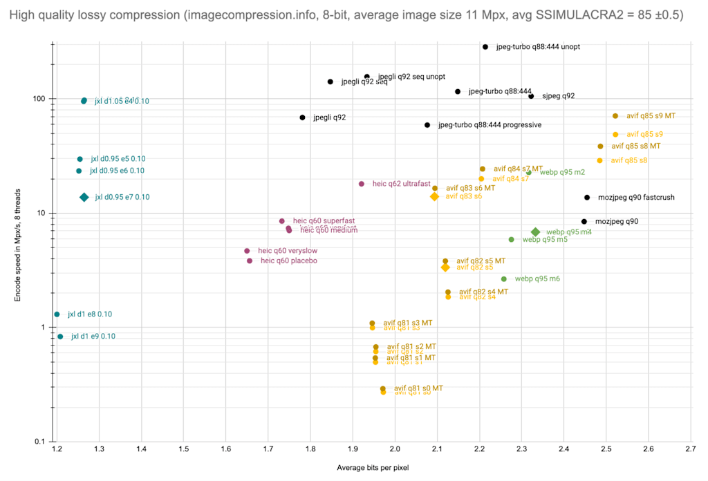
Moving on to the highest quality point that is relevant for the web (corpus average SSIMULACRA2 score of 85, to ensure that most images reach a score above 80), the differences become a little more pronounced.

At this point, mozjpeg no longer beats WebP, though jpegli still does. The Pareto front is now mostly covered by JPEG XL, though for very fast encoding, good old JPEG is still best. At this quality point, AVIF is not on the Pareto front: at its slowest settings (at 0.5 Mpx/s or slower) it matches the compression density of the second-fastest libjxl setting, which is over 100 times as fast (52 Mpx/s).

So far, we have only looked at compression density and encode speed. Decode speed is not really a significant problem on modern computers, but it is interesting to take a quick look at the numbers. The table below shows the same results as the plot above, but besides bits per pixel and encode speed, it also shows the decode speed. For completeness, the SSIMULACRA2 and Butteraugli 3-norm scores are also given for each encoder setting.

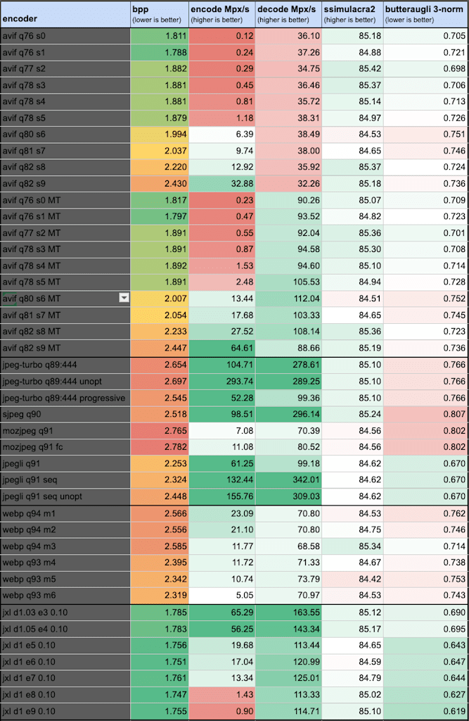
Sequential JPEG is unbeatable in terms of decode speed — not surprising for a codec that was designed in the 1980s. Progressive JPEG (e.g. as produced by mozjpeg and default jpegli) is somewhat slower to decode, but still fast enough to load any reasonably-sized image in the blink of an eye. JPEG XL is somewhere in between those two.

Interestingly, the decode speed of AVIF depends on how the image was encoded: it is faster when using the faster-but-slightly-worse multi-tile encoding, slower when using the default single-tile encoding. Still, even the slowest decode speed measured here is probably “fast enough,” especially compared to the encode speeds.

Finally, let’s take a look at the results for visually lossless quality:

WebP is not on this chart since it simply cannot reach this quality point, at least not using its lossy mode. This is because 4:2:0 chroma subsampling is obligatory in WebP. Also clearly mozjpeg was not designed for this quality point, and performs worse than libjpeg-turbo in both compression and speed.

At their default speed settings, libavif is 20% smaller than libjpeg-turbo (though it takes an order of magnitude longer to encode), while libjxl is 20% smaller than libavif and 2.5 times as fast, at this quality point. The Pareto front consists of mostly JPEG XL but at the fastests speeds again also includes JPEG.

In the plots above, the test set consisted of web-sized images of about 1 megapixel each. This is relevant for the web, but for example when storing camera pictures, images are larger than this.

For a test set with larger images (the same set we used before to test lossless compression), at a high quality point, we get the following results:

Now things look quite different than with the smaller, web-sized images. WebP, mozjpeg, and AVIF are worse than libjpeg-turbo (for these images, at this quality point). HEIC brings significant savings over libjpeg-turbo, though so does jpegli, at a much better speed. JPEG XL is the clear winner, compressing the images to less than 1.3 bpp while AVIF, libjpeg-turbo, and WebP require more than 2 bpp.

While not as dramatic as the improvements in lossless compression, also for lossy compression there have been improvements between libjxl 0.9 and libjxl 0.10. At the default effort setting (e7), this is how the memory and speed changed for a large (39 Mpx) image:

effort setting	memory 0.9.2	memory 0.10	time 0.9	time 0.10	compressed size 0.9	compressed size 0.10	memory reduction	speedup
e7, d1, 1 thread	4,052 MB	397 MB	9.6s	8.6s	6.57 MB	6.56 MB	10.2x	1.11x
e7, d1, 8 threads	3,113 MB	437 MB	3.1s	1.7s	6.57 MB	6.56 MB	7.1x	1.76x

The new version of libjxl brings a very substantial reduction in memory consumption, by an order of magnitude, for both lossy and lossless compression. Also the speed is improved, especially for multi-threaded lossless encoding where the default effort setting is now an order of magnitude faster.

This consolidates JPEG XL’s position as the best image codec currently available, for both lossless and lossy compression, across the quality range but in particular for high quality to visually lossless quality. It is Pareto-optimal across a wide range of speed settings.

Meanwhile, the old JPEG is still attractive thanks to better encoders. The new jpegli encoder brings a significant improvement over mozjpeg in terms of both speed and compression. Perhaps surprisingly, good old JPEG is still part of the Pareto front — when extremely fast encoding is needed, it can still be the best choice.

At Cloudinary, we are actively participating in improving the state of the art in image compression. We are continuously applying new insights and technologies in order to bring the best possible experience to our end-users. As new codecs emerge and encoders for existing codes improve, we keep making sure to deliver media according to the state of the art.