Everything You Need to Know About Compressing Cellular Automata

Cellular Automata are pretty cool things to play with. There are many, many variants, like Conway’s Game of Life, Abelian Sandpiles, Langton’s Loops and Brian’s Brain, but in this blogpost, I’ll just talk about the simplest kinds of cellular automata: one-dimensional cellular automata.

The simplest kind of 1D cellular automata are called Elementary Cellular Automata. They work on a sequence of cells, which can each have two possible states: on and off, or 1 and 0. Starting from an initial sequence, the next sequence is computed based on simple rules: the next state of a cell only depends on the current state of the cell itself and its two neighbors.

For example, here is an elementary cellular automaton called “Rule 22”:

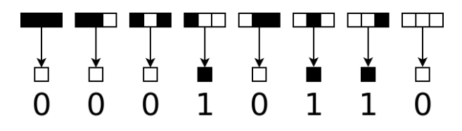
In this automaton, a cell is “on” if in the previous generation, exactly one out of those three cells was on; otherwise it is “off”. Rules can be described using the Wolfram code, which was introduced by Stephen Wolfram. In the case of elementary cellular automata, there are just 8 = 2³ possible configurations of a given cell and its neighbors, and for each configuration there are just two options for the resulting new state, so there are 256 = 2⁸ different elementary CAs, and they can be described using an 8-bit number. So the rules of the diagram above can be described with the binary number 00010110, or in decimal notation: 22.

You can draw the evolution of a 1D cellular automaton (CA) as a 2D image, starting with some initial row of cells at the top and then drawing more and more generations in the rows below it. For rule 22, if you start with just a single black cell in the top row, you get the following image after 512 generations:

Interestingly, the resulting image looks a lot like a Sierpinski triangle. In fact several of the elementary CAs look like this. It is one of the simplest examples of a fractal: the image has a self-repeating structure at different scales.

You might expect that an image with so much repetitive structure in it, generated from such a simple rule, must compress very well. And it does. But it depends on the image format.

As a JPEG, the above image doesn’t compress very well: it weighs 79 KB at quality 90, and that is not even lossless. Even at the lowest possible quality, it is still 16 KB, and at that quality setting, the compression artifacts are quite bad:

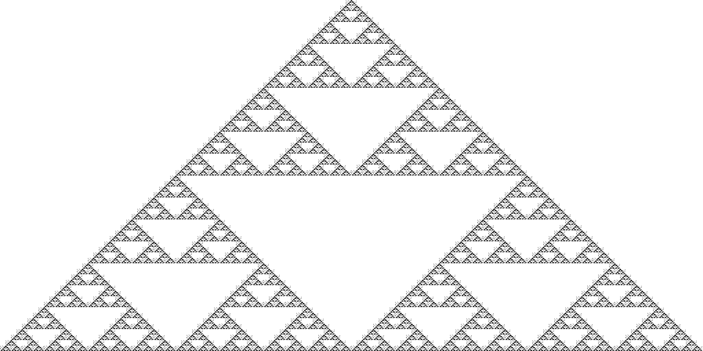
As a PNG however, the image is only 3.4 KB, and that is lossless. So picking the right format can matter a lot, indeed. If you’re using Cloudinary, you don’t have to worry about that: just use f_auto, q_auto (read more) and you will automatically get the most suitable image format and quality settings – in this case, that would be a lossless PNG.

In this example, PNG performs very well because there is a lot of exact repetition in the image. PNG is based on the DEFLATE algorithm, which replaces such exact duplicates by backreferences, saving lots of bytes.

However, not all cellular automata produce such easy-to-compress, repetitive patterns.

For example, Rule 30 produces the following image when starting from a single black cell:

This image weighs in at 215 KB as a quality 90 JPEG, and as a PNG, it is still 24 KB – compared to the 3.4 KB for the Sierpinski triangle image (Rule 22) of the same dimensions, that is quite a jump.

The pattern that rule 30 creates is intriguing: on the left it is repetitive, but on the right, it gets much more chaotic. Triangular structures emerge, but they are positioned in seemingly random ways. Interestingly, in nature there seem to be processes that lead to similar patterns, like on the shell of this Conus textile sea snail:

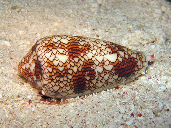
(Image Copyright (c) 2005 Richard Ling, CC-BY-SA 3.0)

PNG performs well for repetitive images like Rule 22, because it “sees” the repetition and encodes it efficiently. It does not “see” the underlying rules of the cellular automaton though, so if those rules lead to chaotic emergent behavior, it gets into trouble. The same is true for GIF and lossless WebP, by the way.

But what if I tell you that there is an image format that can essentially just “learn the rules”, and compress the image very well, regardless of what those rules actually lead to?

Well, the MANIAC entropy coding of FLIF can do just that. It can construct a MANIAC tree that exactly corresponds to the rules of an elementary CA, making sure that each of the 8 configurations of the rules correspond to a different context for the arithmetic coder. Then the probabilities in those contexts will rapidly converge to something very close to 0 or 1, and the encoded bits will have near-zero cost.

For example, the Rule 22 image that was 3.4 KB as a PNG file, is just 83 bytes as a FLIF file. The Rule 30 image that was 24 KB as a PNG, is only 92 bytes as a FLIF.

In fact, those two CA images above (if you have javascript enabled) are actually FLIF files, decoded in your browser using a javascript polyfill called PolyFLIF.

I obtained the smallest FLIF files with the following command-line options for the encoder:

flif -NX1

The option -N causes the encoder to use the non-interlaced variant of the format, so the encoding is top-to-bottom, just like the evolution of the automaton. The default is to do interlacing, which would mean that the encoder cannot “see” the structure since it is encoding pixels from all over the image, resulting in much worse compression. The option -X1 is less important; it allows the arithmetic coder to use more extreme chances (1/4096 instead of the default 2/4096), bringing the “near-zero” cost of the bits even closer to zero.

Here’s an animated plot of the image file size of Rule 22 images with more and more rows, using different image compression formats. Note: the y-axis is logarithmic here!

If you want an even more extreme example, here is a FLIF file that contains a 50 megapixel image of the Rule 30 evolution (5000 rows). Here are the file sizes for that particular image:

 

Amazing how poorly the lossy formats perform on this image, isn’t it? Also rather interesting that PNG and lossless WebP are so close to one another – not that surprising if you know they’re based on similar entropy coding methods, but still. For me however (being the author of FLIF), the nicest thing about the above table is that FLIF beats anything else by a few orders of magnitude :).

Now, of course you shouldn’t draw too many conclusions from something like this. This is an image that is very special in the sense that it represents a best-case scenario for FLIF, while it is quite close to a worst-case scenario for the other formats. It is not that hard to come up with images that turn the tables and compress exceptionally well with, say, PNG or WebP, but compress poorly in FLIF.

FLIF can learn all elementary cellular automata, but it can also handle some more complicated ones. For example, if you allow the next state of a cell to depend not just on the current state of the cell and its neighbors, but also on the previous state of the cell, you get a somewhat different kind of cellular automata that can produce images like these:

Here, I initialized the top row randomly, so the FLIF files are somewhat larger: 269 bytes for the first image, 240 bytes for the second. The corresponding PNG files are 16 KB and 32 KB.

There’s no reason to use only two colors (or states). When using more states, it becomes a bit more tricky to describe the rules concisely, since the number of different automata grows quite quickly; with just 3 states, there are 7,625 billion (3²⁷) automata if you only look at the cell and its two neighbors, and you would need a 27-digit ternary number to describe them.

To simplify things, you can look at totalistic cellular automata, which are a subset of that huge set. In a totalistic CA, the new state depends only on the sum of the current states that are being considered. This forces certain symmetries. For example, the configuration 0,2,1 must result in the same new state as the configuration 1,2,0, or the configuration 1,1,1 for that matter. As a result, you need way fewer digits to specify a totalistic CA. If you have three cell states, the sum can be anything between 0 and 6, and for each of those 7 configurations, there are 3 possible new states, so 7 ternary digits are enough and there are “only” 2187 totalistic 3-color automata.

One of those is Rule 1599, which is my favorite totalistic CA. It looks like this:

Starting from a single “1” cell, Rule 1599 produces this intricate pattern, which goes on for about 8000 rows and then it kind of stops, leaving only a trail of some repeating pattern, about 700 columns wide, that goes on forever. Here is an 899-byte FLIF file that encodes the entire interesting part – it’s a 720×9000 image, so I’m not going to let your browser decode that here.

Take a look at this animated plot of the file sizes:

In this plot, I restricted the number of MANIAC tree learning iterations to just one. You can see that initially the file size grows as the image grows, and it seems to take some time before FLIF “figures out” the rules of the game completely. The file size actually drops while it is learning the rules, and then it very slowly starts to go up again, encoding the extra pixels at near-zero cost. At 3000 rows, the FLIF file is still only 667 bytes, while WebP and PNG are around 140 KB and the lossy JPEG is getting close to 1 MB.

One obvious conclusion from all this is don’t use lossy compression on images of Cellular Automata or in general, on highly structured artificial images with lots of fine details. That’s nothing new, but I think the examples above bring down this point quite nicely.

What’s hopefully new and interesting is that there can be huge differences between different lossless image compression formats. If the format is somehow capable of capturing the “essence” of the image, it might be able to compress it extremely well. For PNG (and lossless WebP), this “best case” scenario is exact repetition. For FLIF, it is harder to describe what the “best cases” are, but Cellular Automata certainly seem to be among them.

Finally, if all went well, this blogpost is actually the first “real” webpage to use FLIF images for purposes other than to demonstrate the javascript polyfill. I hope you enjoyed it!