
The new DNG 1.7 specification allows using JPEG XL as the payload codec to store the raw camera data. This new option became available in flagship phone models like the iPhone 16 Pro and the Samsung Galaxy S24. It brings a much-needed update to the existing compression method that was available in DNG before: lossless JPEG, a not-so-well-known part of the 1993 JPEG standard. According to the estimates by Apple, using a JPEG XL payload reduces the file size of a lossless 48 megapixel ProRAW photo — ProRAW is Apple’s brand name for their own specific flavor of DNG — from 75 MB down to 46 MB. That’s a saving of almost 40%, without any loss.
DNG 1.7 allows storing the image data either losslessly or in a lossy way. Obviously with lossy compression even further gains can be achieved, while still preserving enough fidelity and dynamic range for professional photography. But in this blog post I will focus on lossless compression, and make an attempt at explaining how it actually works.
For lossless compression, JPEG XL uses its so-called modular mode. The other mode is called VarDCT, named that way because it uses the discrete cosine transform (DCT) with variable block sizes and variable quantization. Modular mode is also used as a “sub-bitstream” in VarDCT mode to encode parts of the image data such as the low-frequency signal, which is effectively an 8x downscaled version of the image that gets encoded with lossless compression methods. Lossless JPEG XL does not use VarDCT, but instead encodes the entire image using modular compression.
To understand how it works, let’s first take a look at how lossless JPEG works.
Raster images consist of pixels, which are one big 2D array of sample values that correspond to the light intensity at each position in the image. For grayscale images, there is just one such array; for color images there will be multiple such arrays, typically three (R, G, B) but in case of raw Bayer color filter array data it can also be four (one for each RGGB subpixel in the 2×2 Bayer pattern). These arrays are often called channels, components, or planes.
For simplicity, let’s look at the grayscale case where there is just one channel. The sample values are typically integer numbers. In the case of 8-bit images the range of these numbers is 0 to 255, while in the case of raw camera data, typically 10 to 14 bits per sample are used, so the range can go up to 1023 or 16383. If we have a 1 megapixel 8-bit grayscale image, then we have one million 8-bit numbers to encode.
Without any compression, storing an N-bit number requires, well, N bits. But if the numbers are not completely random, a clever trick can be applied. Assume some numbers occur much more frequently than others, then instead of using the same number of bits for each number, entropy coding can be applied. The basic idea is to use a code that assigns a shorter sequence of bits to represent the numbers that are more frequent, and a longer sequence to the numbers that are rare. Just like how Morse code uses a shorter code for common letters like E ( ▄ ) and T ( ▄▄▄ ) than for less frequent ones like Q (▄▄▄ ▄▄▄ ▄ ▄▄▄) and X (▄▄▄ ▄ ▄ ▄▄▄).
In lossless JPEG, Huffman coding is used as a method for entropy coding. In essence, this works by first describing a histogram that gives the frequency of each number, constructing a prefix code based on that histogram, and then using that code to represent the data. In prefix coding, no code can start with something that can also be interpreted as another (shorter) code. Prefix codes have the advantage that they work without ‘spaces’. In Morse code (which is not a prefix code), to distinguish the letter A ( ▄ ▄▄▄) from the letter E ( ▄ ) followed by the letter T (▄▄▄), the individual codes have to be separated by a short gap. Digital files are one long stream of bits without any gaps — but prefix codes, by design, don’t require a separation between the codes, since no ambiguous sequences can be created in the first place.
For example, suppose the numbers 0, 1, and 2 are much more common than the numbers 3 to 255. Say 30% of the numbers are 0, another 30% is 1, yet another 30% is 2, and the remaining 10% is evenly divided among the remaining numbers. Then instead of using 8 bits for each number, you could use 2-bit combinations (00, 01, 10) for the common numbers and 10-bit combinations (11xxxxxxxx) for the rare numbers. If you then have one million numbers, instead of 1 MB (one million times 8 bits), you would only need 350 kB (900,000 times 2 bits plus 100,000 times 10 bits).
But by itself, this is not enough for image compression. The histogram of the sample values themselves will typically not allow effective entropy coding, since all possible values will occur with a more or less similar frequency. Here’s where the second clever trick comes into play: prediction.
Instead of storing the sample values themselves, what is stored are the residuals after prediction. The assumption is that often, sample values will be similar to the values at neighboring positions. For example, a predictor that is used in lossless JPEG is “West plus North divided by two”, or in other words, the predicted value is the average of the sample value above (North) and to the left (West). Then instead of storing the sample value itself, the difference between the actual sample value and the predicted value is stored. This is called the residual, and it will be zero if the prediction was exactly right.
Using prediction, we can change the distribution of numbers from something that looks like the histogram on the left, to something that looks like the histogram on the right:


The more unequal the histogram, the better entropy coding will work. Fewer bits can be used for the more frequent numbers, and the end result is a smaller file.
In lossless JPEG, that’s pretty much it. You can choose a predictor, replace the image data with the predictor residuals, and encode those with Huffman coding where values close to zero (well-predicted pixels) will end up using fewer bits. Here is an illustration of the process:

PNG uses basically the same principle, with two tweaks that make it more effective, especially for non-photographic images. The first tweak is that you can change the predictor for every horizontal row of the image. For example, in the first few rows maybe the simple West predictor works best (using the value of the pixel on the left as the predicted value), while on the next rows the North predictor works best.
The second tweak is that it adds special codes that represent repetition. Basically these codes allow an encoder to give an instruction to the decoder: “for the next N residuals, copy/paste the numbers you just decoded, starting at a position X numbers ago”. This “copy/paste instruction” mechanism is known as LZ77, and the combination of LZ77 with Huffman coding is known as the DEFLATE algorithm. It is not only used in PNG but also in general-purpose compression methods like ZIP or gzip.
The basic idea of lossless JPEG XL, i.e. modular mode, is similar: prediction is applied, and then the residuals are entropy coded. Except everything is a lot more sophisticated.
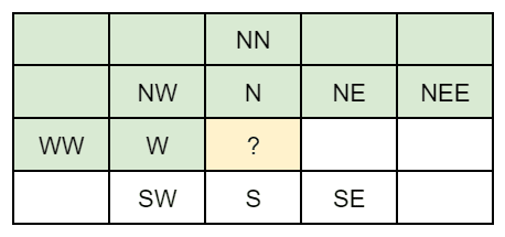
There are more predictors available in JPEG XL than in other lossless codecs. Predictors are always based on already-decoded sample values. In nearly all codecs, images are processed top to bottom, left to right (a notable exception being FLIF), so when predicting the value at the question mark (?), the samples indicated in green can be used:
This table lists all the predictors that can be used in various lossless codecs:
| Predictor | JPEG Lossless | PNG | WebP Lossless | FFV1 | FLIF | JPEG XL Lossless |
| Zero (no predictor) | ✔ | ✔ | ✔ | ✔ | ||
| W | ✔ | ✔ | ✔ | ✔ | ||
| N | ✔ | ✔ | ✔ | ✔ | ||
| WW | ✔ | |||||
| (W+N)/2 | ✔ | ✔ | ✔ | ✔ | ||
| W+(N-NW)/2 | ✔ | |||||
| N+(W-NW)/2 | ✔ | |||||
| Paeth (W, N or NW, closest to W+N-NW) | ✔ | |||||
| Select (abs(N−NW) < abs(W−NW) ? W : N) | ✔ | ✔ | ||||
| W+N-NW | ✔ | ✔ | ||||
| W+N-NW, clamped to min(W,N)..max(W,N) | ✔ | ✔ | ✔ | |||
| NW | ✔ | ✔ | ✔ | |||
| NE | ✔ | ✔ | ||||
| (W+NW)/2 | ✔ | ✔ | ||||
| (N+NW)/2 | ✔ | ✔ | ||||
| (N+NE)/2 | ✔ | ✔ | ||||
| (W+NW+N+NE)/4 | ✔ | |||||
| (N+(W+NE)/2)/2 | ✔ | |||||
| (6 * N − 2 * NN + 7 * W + WW + NEE + 3 * NE + 8) /16 | ✔ | |||||
| Predictors involving S, SW, SE | ✔ | |||||
| Self-correcting (Weighted) Predictor | ✔ |
The most useful predictors of earlier codecs were included in JPEG XL’s modular mode, and additionally three new predictors were added that are unique to JPEG XL — one of which we’ll discuss in more detail later.
The biggest innovation however is that all of these predictors can be combined much more effectively. Instead of using just a single predictor like in JPEG lossless and FLIF, or a fixed predictor per row as in PNG, or even a predictor per macroblock as in WebP lossless, predictors can be changed on a per-pixel basis in JPEG XL.
To know which predictor to use, a decision tree (called the MA tree, for ‘meta-adaptive’) is used. This tree is signaled in the compressed bitstream, so a different tree can be used for each image. The MA tree has decision nodes that ask a question about neighboring sample values, e.g. “Is the sample above the current position larger than 50?” (“N > 50”) or “Is the sample value on my left larger than the sample value to the left of that value?” (“W-WW > 0”). The questions can also be about the current (x,y) position, or about sample values at corresponding positions in previously decoded channels.
The leaves of this decision tree then say which predictor to use in each case. Additionally there can be a multiplier and an offset: the residuals will first be multiplied by this multiplier before adding them to the prediction and then adding the offset.
Instead of using just a single histogram, multiple histograms can be used. Each leaf of the MA tree also has its own histogram. The idea of using different histograms in different situations is called context modeling and it’s not new: it has been widely applied in various compression methods, including video codecs as old as H.264, but also for example Brotli and WebP lossless. What’s new though is that the context model itself is not fixed, but it is signaled as part of the bitstream. While a fixed context model allows adaptive entropy coding (using histograms adapted to the local context), in JPEG XL the context model itself can also be adapted to the specific image data that is being encoded, hence it’s called meta-adaptive context modeling.
The context map in Brotli and the prediction and entropy images in WebP lossless are a simple, fixed-complexity and fast-to-decode approach to context modeling. The more flexible context modeling with meta-adaptive (MA) trees was first implemented in FLIF, but its adaptive probability distributions had an impact on decoding speed. The best of both of these approaches were combined in JPEG XL’s modular coding. Consequently, static distributions give an advantage to JPEG XL in decoding speed due to the elimination of dynamic decode-time updates, while it still benefits from the flexibility of MA trees. Furthermore, JPEG XL allows for histogram sharing between leaf nodes in its MA trees, a feature absent in FLIF where each leaf node corresponds to a unique context. This shared histogram approach, reminiscent of the context map concept, avoids redundant encoding of similarly shaped histograms. Finally, JPEG XL extends the role of the MA tree beyond context definition to include predictor selection, a function not present in FLIF’s MA trees.
If we take the same small example image from before, using JPEG XL’s modular mode, the encoding could look like this:

The ability to switch between predictors depending on the local context helps to make the prediction residuals smaller; the ability to use different histograms in each context helps to make the entropy coding more effective.
Speaking of entropy coding: this also is one of the things where JPEG XL made improvements. While lossless JPEG (and PNG, for that matter) use Huffman coding, JPEG XL offers two options. Huffman coding is still possible (it does have one advantage: it is more convenient for very fast encoding), but alternatively, ANS coding can be used. Also, like in PNG and WebP lossless, LZ77 “copy/paste” instructions can be used in JPEG XL too.
In Huffman coding, as soon as there are two or more different symbols to encode, the minimum code length is 1 bit. All codes use an integer number of bits, which means the distributions can only be approximated. For example, suppose there is a distribution with only three possible values, each with the same probability ⅓. In Huffman coding, the best you can do is assign a one-bit code to one of the symbols and a two-bit code to the two other symbols — but that would be an optimal code for a distribution of {50%, 25%, 25%}, not for the actual distribution. ANS coding is a more sophisticated entropy coding method that effectively allows using “fractions of a bit”, allowing better compression since the distributions can be approximated much more accurately.
This is particularly important since context modeling can lead to some contexts that correspond to regions of the image that are particularly well-predicted (e.g. patches of a smooth sky), so the histogram of the residuals in these contexts could for example have 90% zeroes. With Huffman coding you have no choice but to still use 1 bit for every zero (effectively “rounding” the 90% down to 50%), while ANS coding allows using less than 1 bit per sample.
In fact, in some contexts, the histogram could even be a singleton: literally all of the residuals occurring in that context have the same value (typically the value zero). In the JPEG XL variant of Huffman coding and ANS coding, this ‘pathological’ type of histogram is well-covered: it leads to asymptotically zero bits being used per residual. That is, the only thing that needs to be signaled is the singleton value, and then no matter how many residual values have to be encoded, no further bits have to be used.
This leads us seamlessly to JXL art — impressively tiny JPEG XL files that somehow decode to interesting images. They are effectively an image constructed in such a way that all the prediction residuals happen to be zeroes, which means all the MA tree leaves can point to the same singleton histogram saying “100% probability of zero”, and thus no matter how many pixels are in the image, no further bits are needed. The only thing the JPEG XL file effectively contains are some bytes with header information, followed by a description of an MA tree, followed by millions of… zero-bit codes.
Schematically, it looks like this:

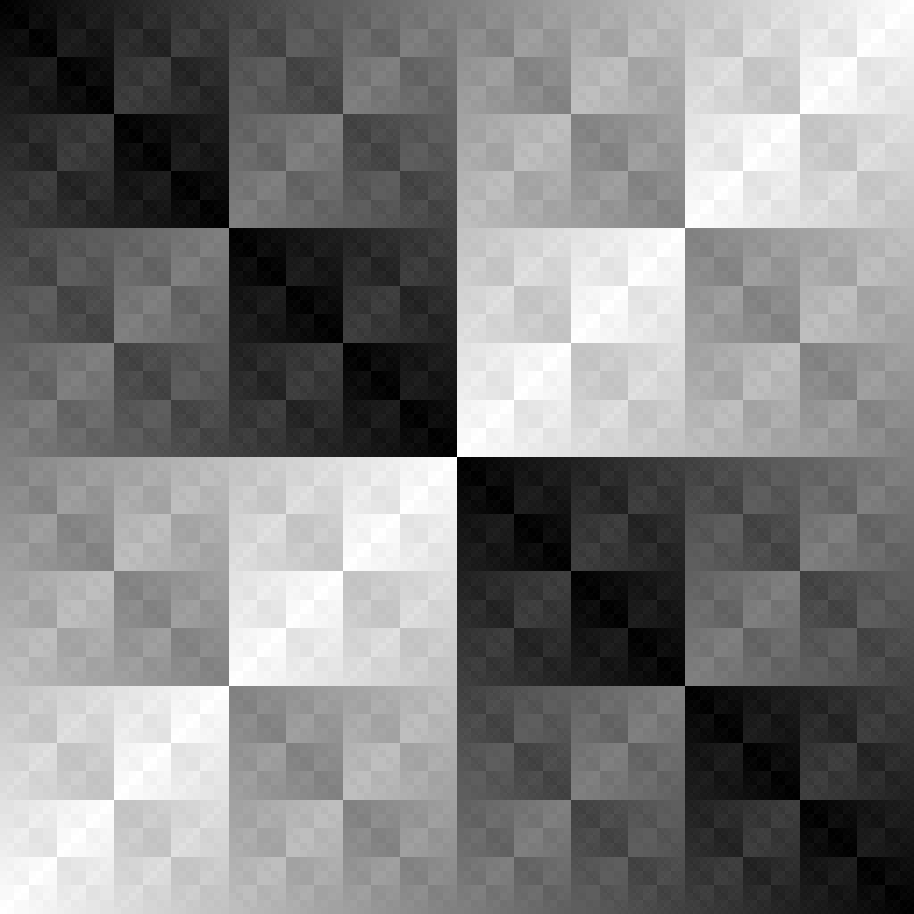
There’s an online tool available in case you want to experiment with this. Even small MA trees can produce surprising images. For example, this image (also known as the XOR pattern) can be represented as a 25 byte jxl file:
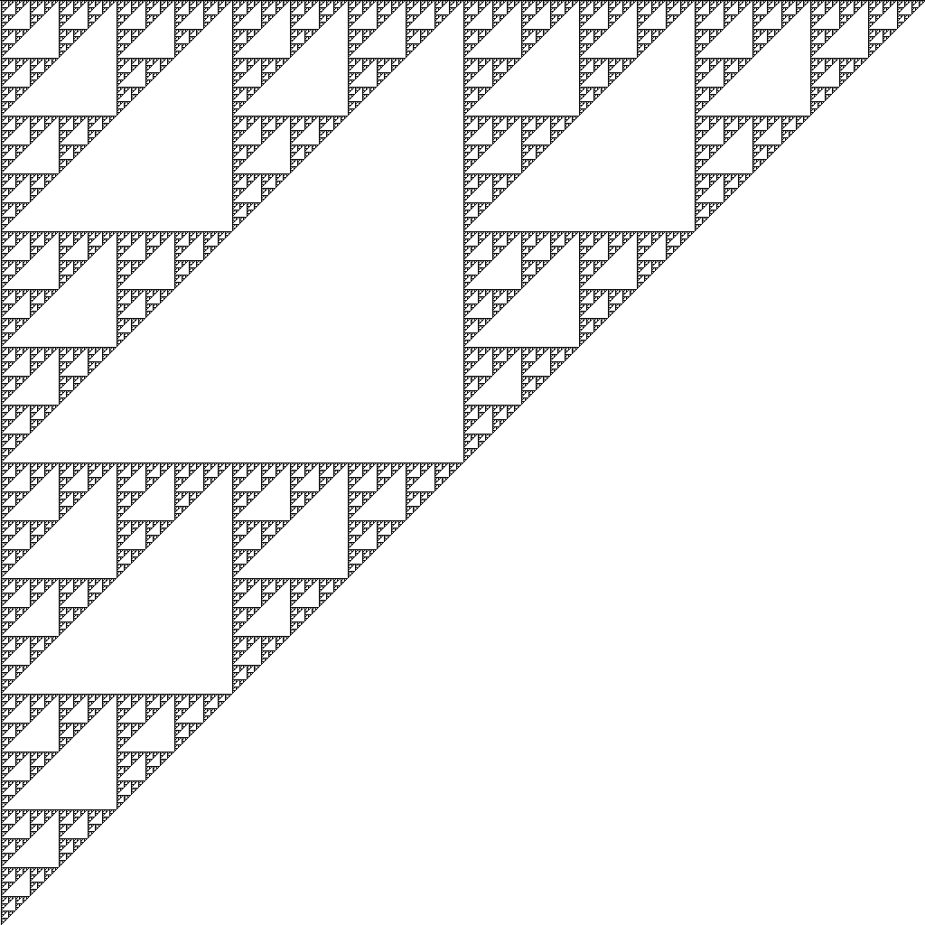
This Sierpinski triangle can be done in only 23 bytes:
Obviously such small file sizes are not representative of what will happen for real images that are not specifically constructed to result in best-case entropy coding. But it does demonstrate the expressivity and flexibility of meta-adaptive context modeling of JPEG XL’s modular mode.
In lossless JPEG — and also in PNG, WebP lossless and FLIF — the only predictors that are available are relatively simple ones: use the value above or to the left, the average of those two, etc. In JPEG XL these simple predictors are also available. But JPEG XL adds some new predictors, one of which is very sophisticated and worth diving into. It is called the self-correcting predictor, also known as the weighted predictor. It works as follows.
There are four different “sub-predictors”, which are parameterized (the constants in their formula can be signaled). One of them is just a simple predictor (W + NE – N), but the three others have terms in them that make them ‘self-correct’: the prediction algorithm keeps track of the prediction errors in the previous row of the image, and these errors are then fed back into the new predictions. This feedback loop causes the predictor to automatically correct its past mistakes, to some extent.
For each of the four sub-predictors, the algorithm keeps track of its performance in the recent past. Weights are updated that reflect the current accuracy of each sub-predictor. The final prediction is then a weighted average of the sub-predictions, where the currently best-performing sub-predictor has the largest impact on the final prediction. This is an additional way in which the overall predictor is self-correcting.
As part of the bookkeeping to compute this predictor, a very useful value called max_error is maintained, which gives an indication of how well the self-correcting predictor is performing in the current region of the image. This value can be used in decision nodes of the MA tree and is often effective for context modeling. For example, when max_error is low, it will be good to use histograms that assign high probabilities to residual values close to zero, while if max_error is high, it will be likely that the prediction is wrong so lower probabilities should be given to low-amplitude residuals.
Especially for photographic images, including the application of JPEG XL in DNG 1.7, this self-correcting predictor has proven to be very useful. At the low encoding effort setting 3 (–effort=3) of libjxl, in fact only the self-correcting predictor is used, with a fixed MA tree that only uses the value of max_error in its decision nodes. Compression can be improved by exploring more predictors and more generic MA trees (which requires spending more encode effort), but this low-effort encode setting already outperforms many other lossless compression formats for photographic images.
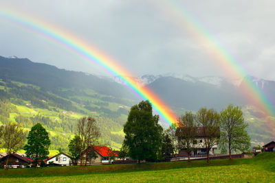
In JXL art, the self-correcting predictor can be used to produce quite interesting, natural-looking images, such as this 124-byte jxl image:

For grayscale photographic images, the coding tools described above are the most important ones. But there’s more to be discussed. After all these explanations, one question hasn’t been answered yet: what is it that is modular about the modular mode? Why do we call it that??
Part of the reason for this name is something that has been mentioned already: modular encoding is not only used in lossless JPEG XL, but also as a sub-bitstream in various parts of the lossy VarDCT mode. In that sense, it acts like a submodule. It is used for all kinds of image-like data, including the 8x downscaled low frequency image, signaling of local smoothing filter strengths, weights for adaptive quantization, factors for chroma-from-luma, and quantization tables.
But there’s another reason. Modular encoding allows reversible transformations to be applied to the image data before encoding it, to make compression even more effective. These transformations can be chained in arbitrary ways — the list of which transformations to apply and in what order gets signaled in the bitstream so the decoder can do the appropriate inverse transformations to restore the original image data. In a way, they are like LEGO bricks that can be composed in various ways, which is a rather expressive and, well, modular way of encoding image data.
So far, we have only discussed how a single channel of image data gets compressed. Color images have three channels though (RGB), and JPEG XL also supports additional channels for alpha transparency, depth maps, selection masks, spot colors and any other kind of “extra channels”. These channels can simply be encoded independently, but encoding them this way misses out on opportunities to exploit the fact that very often, the data in the different channels is strongly correlated: the image data in each of the three RGB channels tends to be quite similar.
One of the modular transforms is called RCT, short for Reversible Color Transform. It takes three channels as input, and applies a mathematically reversible operation on them that can help to decorrelate the image data. Several RCTs are defined, one of them being the YCoCg-R transform. The resulting transformed channels can be compressed better since some of the redundancy between channels gets eliminated.

Another modular transform is called Palette. It is particularly useful for non-photographic images that only use a limited number of different colors. It takes any number N of channels as input (for example N=3 for RGB, or N=4 for RGBA), and replaces them with two new channels: one that encodes the palette and one that encodes the indices. The palette is effectively a numbered list of N-channel colors, which is represented as a nb_colors x N image (where nb_colors is the number of colors in the palette). The other channel represents the actual image data, using just a single channel instead of N channels, where the numbers do not represent sample values, but indices referring to colors in the palette.
PNG, WebP lossless, and GIF also support palette coding, but the Palette transform of JPEG XL is more powerful, in various ways. The most obvious difference is that nb_colors is not limited to 256, but larger palettes are also allowed. Another difference is that the number of channels to apply Palette to is arbitrary. Even the N=1 case can be quite useful, especially for high bit depth images, where it can happen that not all possible sample values actually occur in the image. In that case, mapping the larger range to a smaller range can be beneficial for compression.
Yet another difference is that the Palette transform comes with “default colors”: whenever the index channel uses a number that exceeds the number of colors in the palette, this is treated as a reference to a default color. This means that even a “zero-color” palette (one that does not require any signaling of the palette colors) can be useful, potentially saving some bytes for small images like icons.

The biggest difference however is that the Palette transform also defines Delta palette entries. These are “relative palette colors”, that do not correspond to a specific color, but rather to a difference of colors, in particular, the difference between the predicted color (according to one of the predictors) and the actual color. For example, a delta entry (0,0,0) would mean “use the predicted sample values”, while a delta entry (-1,0,2) means “use the predicted sample values, and subtract 1 for R, keep G as predicted, and add 2 for B”. This is a powerful mechanism that is particularly well suited for near-lossless encoding using a palette approach without suffering from the usual problems of a limited number of colors. Smooth gradients can be encoded very nicely using delta palette entries, instead of having to use dithering as would be the case in PNG8 or GIF. Finally there are also default delta palette entries: if the index channel refers to negative indices, these are treated as a reference to the default delta palette.
Both the RCT transform and the Palette transform can be applied globally to the entire image, but they can also be used locally. By default, JPEG XL encodes the image in tiles of 256×256 pixels (also called groups). These tiles can be encoded and decoded independently, which enables multi-threaded implementations and efficient cropped decoding (decoding only a specific region of the image), both of which are useful when dealing with large images. But it also means that each group can select its own local transforms to be applied on top of the global transforms. For example, it could be the case that the entire image can be represented using a 500-color palette, so it will likely be beneficial to do the Palette transform globally. But then in a specific group (corresponding to one 256×256 region of the image), it could be the case that only 50 out of these 500 colors are actually used. In that case, it will likely be a good idea for an encoder to use an additional local Palette transform — one that operates only on a single channel, since at this point the image has already been reduced to a single channel containing indices. That way, the range of the indices can be reduced from 0..499 down to 0..49, allowing better compression.
Finally, there’s a third type of transform called Squeeze. Its basic step is to take a channel and replace it with two new channels where one of the dimensions (horizontal or vertical) has been halved. The total number of samples remains the same, and this transform is reversible. The first new channel is effectively a downscaled (“squeezed”) version of the image, while the second new channel contains the residuals needed to losslessly reconstruct the original-resolution image. This step can be applied several times, each time splitting the data into a low-frequency signal and residuals representing the high-frequency information. It has the advantage of allowing progressive decoding by storing the lower frequency information first, thus allowing a decoder to show downscaled versions of the image even when only part of the jxl file has been transferred.
While the Squeeze transform can be used for lossless encoding, its main application is in lossy encoding: by quantizing the high-frequency residuals (e.g. by using a multiplier > 1 in the MA tree and reducing the precision of the residuals accordingly), a kind of lossy compression can be applied.
Both the Squeeze transform and the Delta Palette transform can be used to do lossy compression without any use of the DCT. While for lossy compression, VarDCT mode generally produces the best results (which is why it is the default choice for lossy in libjxl), this does introduce two new ways of doing lossy compression, both within the modular mode of JPEG XL.
 original image, 163 kB PNG |
 |  |
 reduced to 100-color palette, 39 kB PNG |  |  |
 lossy modular using Delta Palette, 37 kB JXL |  |  |
 lossy modular using Squeeze, 37 kB JXL |  |  |
 VarDCT mode, 37 kB JXL VarDCT mode, 37 kB JXL |  |  |
All in all, JPEG XL’s modular mode is a very expressive and versatile image (sub)codec that offers a lot of powerful coding tools. The current libjxl encoder implementation can make effective use of most of these coding tools, but it will probably take years if not decades to unlock the full potential of all coding tools in JPEG XL. Even for JPEG and PNG, which are comparatively much less expressive, it took two decades to arrive at state-of-the-art encoders such as MozJPEG, Jpegli, and ZopfliPNG.
So there’s clearly still room for encoder improvements in JPEG XL too. But even as it is now, the compression gains that can be achieved with current JPEG XL implementations — like the one in the iPhone 16 Pro — are substantial. If you’ve read all the way through here, you’ll now better understand where these gains are coming from. And who knows, maybe you will be inspired to create an even better encoder for JPEG XL!