Obtaining the optimal balance between image quality and file size is one of Cloudinary’s core products. We aim for high-quality images alongside small bandwidth. A good balance between image quality and file size is critical to user experience. For instance, consider the case of e-commerce platforms that rely on high-quality product images to drive sales but also fast page loading to not lose users tired of waiting. 

In this series, we’ll share our endeavors on building a whole new AI-based solution of image optimization based on the human perception of image quality.

Since an AI is only as good as the data it was trained on, in this first part, we’ll deep dive into how we collected data for training this new image optimization AI engine.

Compressing images to tiny file sizes while still preserving the original high quality is easy nowadays thanks to modern image compression codecs like WEBP, AVIF, and good old JPEG.

However, building an image optimization engine to use these modern compression algorithms properly is the tricky part. Effective image optimization, in terms of quality and bandwidth, essentially means knowing the exact amount of compression that can be applied to an image to minimize its file size without losing quality. In order to do that, one would need some kind of rule or heuristic to assess image quality. It needs a metric, specifically an IQA (image quality assessment) metric. A robust IQA can be used to drive this image optimization engine, choosing formats, settings, compression magnitude, etc. 

People have researched IQA metrics before, so why not use them?

Well, indeed there are both many modern and classic IQA metrics, but none of them suits our scenario. These metrics are built and developed considering all sorts of different distortions and artifacts but almost none corresponding to image compression. Hence, the only option was to create our very own new IQA metric. One that would be aware of compression-related issues, nuances, and how they translate to human perception of image quality 

Developing this AI-based IQA metric required an appropriate dataset for training and evaluation. But what we considered to be a relatively straightforward step, turned out to be a significant milestone that required quite a lot of thinking and research. 

Like any other computer vision dataset, the first step would be gathering a representative set of images. You want this set to be diverse enough and the images to be pristine enough and this isn’t too difficult to find using popular stock image platforms like Getty or Pexels. 

The next thing we did was encode/compress these images using all sorts of image encoders. In order to span the quality spectrum, we used many different encoders with different settings, both old and modern, popular and niche, on the set of original images.

At Cloudinary, we share a considerable number of resources in this field, which you can explore further through our various blog posts, publications, and documentation.

But given these images and the many corresponding compressed variants, how do we assign them with quality scores? We need actual numeric quality values aligned with human perception. 

There are many IQA papers out there and all of them use some paradigm of annotating image quality. 

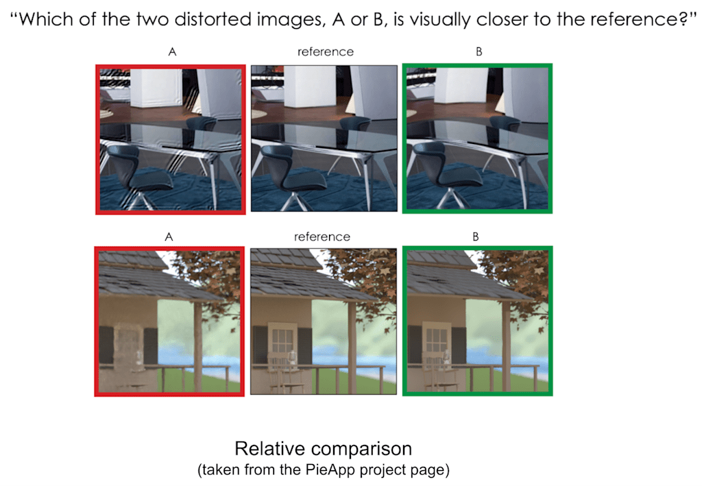
PieApp and PIPAL (and later on CVPR NTIRE workshops) follow the relative comparison annotation approach. In this approach, many pairs of images are compared using human annotators. Then, all these comparisons are aggregated together into a single “leaderboard.” Each image is given a score according to how many “games” it won.

This approach enjoys the advantage of being simple as the user only needs to choose the better-looking image from a given pair. Its major disadvantage though, is not having a strict mapping to a fixed range of values. Consider a set of pairs comparison, even the image given the lowest score might still be of great quality. It just happens to be slightly worse than all the other images.

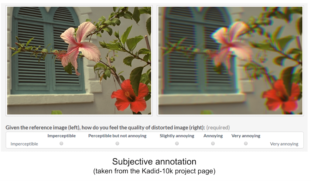
Other approaches use subjective annotation, also known as the mean opinion score (MOS) annotation, a popular method used by many datasets (Kadid10k, NIMA, etc.). It’s a simple concept yet difficult one to execute as shown by this great paper. To make a long story short, MOS annotation is both expensive and noisy. Despite that, this approach has the benefit of being entirely based on the human perception of quality.

We decided to combine these paradigms in building our IQA corpus. The MOS part will help us anchor our dataset to the human perception of appeal while the relative comparison part will be used to truly grasp all the nuances that differentiate between images.

At this point, all that’s left is to submit the annotation process to some crowdsourcing platform.

In order to perform effective AI training, you want your data to be as accurate as possible. That’s why the first thing we did upon getting the annotations from the platform was to explore our new dataset. We built UI tools to analyze different statistics, verified prior assumptions, and learned new things regarding human perception and how it’s affected by different compression settings. 

We also discovered quite a few issues/problems related to the accuracy of the annotations. 

Any AI practitioner knows that everything depends on data quality, even the strongest architecture will fail dramatically if trained with bad ground truth. 

Unfortunately, in crowdsourcing platforms, there’s always the chance of rogue participants entering your task. Such users inject a lot of noise into the ground truth annotations that may prevent accurate training of the model. 

As said, our goal is to explore the entire span of image quality and how it’s affected using different compression settings. This task is quite easy when dealing with either clearly good or clearly poor quality. Since most users are doing a decent job, the existence of rogue users doesn’t dramatically affect the score of such images. However, when dealing with mid-quality images, this isn’t the case. Being mid-quality, there isn’t a clear consensus about these images’ quality, so having large enough rogue users annotating them makes it impossible to get an accurate quality score.

Considering the example below, the first and second images MOS seems reasonable considering the scores histograms. However, the MOS assigned to the last image, which is of medium quality, doesn’t seem right as there are clearly two different opinions on the image quality, and none of them are 5.5.

We understand that we must remove rogue users from the annotations, but how can we detect them?

Well, some of them were pretty easy to detect using predefined tests hidden in the annotation tasks like grading pristine images or grading the same image twice. This simple practice can point to participants that should be removed from the corpus.

Besides hidden tests, we also analyzed each individual participant profile according to its annotations and how they compare with other participants. The general idea is rogue users doing random annotations will always be in severe disagreement with all the other participants regarding the images they graded. 

To clarify, for each individual participant, we calculated the difference in MOS units between the scores they assigned to images and the average scores given by all other participants for those same images. Subsequently, we represented each participant by the average and standard deviation of these differences and mapped them onto a 2D grid.

This figure was enlightening and revealed different types of participants. We marked each group threshold (obtained through ablation) using the black dashed lines.

• Random voters. These participants’ profiles indicated they were constantly in significant disagreement with all the other users. They were just randomly clicking their way through the annotation task. 
• Binary voters. In general, these participants are on par with all the other participants but according to their std, they only give either very low or very high scores. Clearly not putting the effort into really assigning accurate scores to the images.
• Biased users. In agreement with the general opinion but according to their mean distance, these users have a tendency to be either too forgiving or too judgemental compared to the other users.
• Quality users. These are the users who took their job seriously and were always in consensus with the general opinion.

Given these insights on the different participants profiles coexisting in the dataset, we did the following:

• Removed random and binary voters, nothing to very little that we can learn from these participants’ annotations.
• Normalized slightly biased users, this small calibration can help a lot in reducing variance in the annotations.

The impact of these steps was clear when viewing disputed testcase, like in this example:

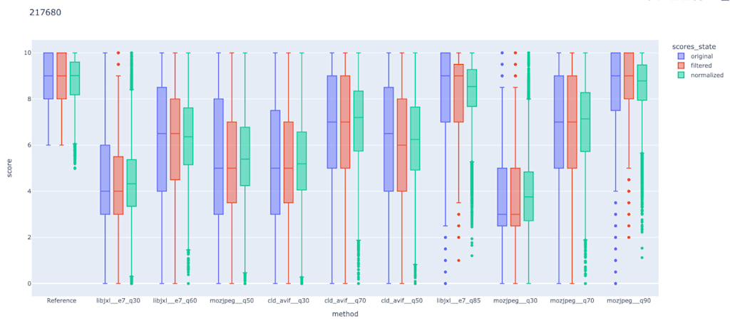
But also when viewing the score distributions of different compression settings, we noticed they had a smaller variance than before, indicating that true noise was removed.

In the next article, we’ll share more about how we trained the IQA model using both types of annotations, subjective and relative, and what we were able to achieve using the learned IQA metric.

Want to discuss the topic of this blog in more detail? Then head over to Cloudinary Community forum and its associated Discord to get all your questions answered.