Image Segmentation Python: The Complete Guide

Image segmentation is a foundational technique in modern computer vision, powering applications from medical imaging and satellite analysis to retail automation and document processing. Rather than treating images as raw pixel grids, segmentation enables us to understand structure, boundaries, and objects at a much deeper level. Python has emerged as the dominant language for this work, thanks to its rich ecosystem of scientific, vision, and deep learning libraries.

In this guide, we walk through image segmentation in Python from fundamentals to production-ready workflows. We cover classic rule-based techniques, modern deep learning models such as U-Net, Mask R-CNN, and transformers, and practical evaluation strategies. We also explore when cloud-based solutions like Cloudinary can simplify large-scale segmentation pipelines by removing the burden of model management and infrastructure.

Key takeaways

• Image segmentation focuses on understanding what is where in an image, not just what objects exist.
• Traditional techniques like thresholding and region analysis remain useful in controlled environments.
• Deep learning models provide higher accuracy and robustness for complex, real-world scenes.

In this article:

• What Image Segmentation Is and Why Python Is a Great Fit
• Setting Up: Installing scikit-image, OpenCV, PyTorch, TensorFlow & Transformer
• Segmentation Basics in Python: Thresholds, Clustering, and Region Growing
• Classic Segmentation Pipelines with scikit-image and OpenCV
• Modern Deep Learning Approaches: U-Net, Mask R-CNN, and Transformers
• How to Evaluate Segmentation: IoU, Dice, Precision/Recall, and Visual Debugging
• Efficient Image Segmentation with Cloudinary

What Image Segmentation Is and Why Python Is a Great Fit

Image segmentation is the process of dividing an image into meaningful regions, assigning each region a label based on its content. Instead of treating an image as a single grid of pixels, segmentation lets us separate objects, boundaries, or areas of interest.

For example, we might isolate a tumor from a medical scan, extract roads from satellite imagery, or split text and graphics in a scanned document. In practice, segmentation converts raw images into structured data that downstream systems can reason about.

There are different levels of image segmentation. Some tasks only need basic foreground–background separation, while others require precise pixel-level masks for multiple objects in the same image. Classic approaches rely on rules such as intensity thresholds, color similarity, and edge detection. Modern approaches use deep learning models that learn complex shapes and context directly from data.

Regardless of the technique, the goal stays the same: understand what is where in an image, not just what the image contains.

Why Use Python for Image Segmentation

Python is an excellent fit for image segmentation because it sits at the intersection of scientific computing, computer vision, and machine learning. Libraries like NumPy give us fast array operations for pixel data, while tools such as scikit-image and OpenCV provide well-tested implementations of classic segmentation algorithms.

On top of that, deep learning frameworks like PyTorch and TensorFlow enable the training and deployment of state-of-the-art segmentation models with relatively little boilerplate code. This ecosystem enables us to move from experimentation to production without switching languages or rewriting pipelines.

Another reason Python works so well is its ease of integration with real-world workflows. We can load images from disk, preprocess them, train a model, evaluate the results, and deploy the same logic via an API or a batch job.

Setting Up: Installing scikit-image, OpenCV, PyTorch, TensorFlow & Transformer

Before we start building segmentation pipelines, we need a solid Python environment with the right libraries installed.

Installing Core Image Processing Libraries

We will start with the two libraries that cover most classic segmentation workflows.

• scikit-image is built on NumPy and SciPy and provides a clean, Pythonic API for tasks like thresholding, region labeling, morphology, and feature extraction.
• OpenCV focuses on performance and low-level computer vision operations. It’s widely used for preprocessing, contour detection, filtering, and real-time pipelines.

Install both with pip via pip install scikit-image opencv-python

Installing Deep Learning Frameworks

Modern image segmentation often relies on neural networks, especially for complex scenes or pixel-level accuracy. The two most popular Python frameworks are PyTorch and TensorFlow.

• PyTorch is widely used in research and production for segmentation models like U-Net, Mask R-CNN, and transformer-based architectures. Its dynamic computation graph makes debugging and experimentation easier.
• TensorFlow and its high-level Keras API are commonly used in production environments and provide strong tooling for training, exporting, and deploying segmentation models.

These can be installed via pip as well with these commands:

pip install torch torchvision torchaudio
pip install tensorflow

Installing Transformers for Modern Segmentation Models

Transformer-based models are now standard in image segmentation, especially for tasks that require global context. Libraries like Hugging Face Transformers provide ready-to-use implementations of vision transformers, segmentation heads, and pretrained checkpoints.

Install the Transformers library with pip install transformers

For many segmentation workflows, Transformers is used together with PyTorch, so having both installed is essential.

Verifying the installation

After installing everything, it’s a good idea to confirm that the libraries are available and imported correctly. Open a Python shell and run the following imports:

import cv2
import skimage
import torch
import tensorflow as tf
import transformers

print("OpenCV:", cv2.__version__)
print("scikit-image:", skimage.__version__)
print("PyTorch:", torch.__version__)
print("TensorFlow:", tf.__version__)
print("Transformers:", transformers.__version__)

With the environment set up, we are ready to move on to segmentation fundamentals.

Note: The complete code for this article is available in this Google Colab Notebook.

Segmentation Basics in Python: Thresholds, Clustering, and Region Growing

Before moving to full pipelines or deep learning models, it’s worth understanding the core segmentation techniques that underpin most workflows. These methods are straightforward, fast, and still widely used in production systems where images are controlled and well-defined.

Threshold-based Segmentation

Threshold segmentation separates pixels based on intensity values. It works best when there is a clear contrast between foreground and background, such as scanned documents, microscopy images, or high-contrast scenes.

A common approach is Otsu’s method, which automatically selects a threshold from the image histogram.

import matplotlib.pyplot as plt
from skimage import io, filters
## image link: https://pixabay.com/photos/miniature-model-fire-fighters-road-4308104/
image = io.imread("/content/miniature-4308104_1280.jpg", as_gray=True)
threshold = filters.threshold_otsu(image)
binary = image > threshold

plt.figure(figsize=(10,6))
plt.subplot(1, 2, 1)
plt.title("Original")
plt.imshow(image, cmap="gray")
plt.axis("off")
plt.subplot(1, 2, 2)
plt.title("Thresholded")
plt.imshow(binary, cmap="gray")
plt.axis("off")
plt.show()

Output:

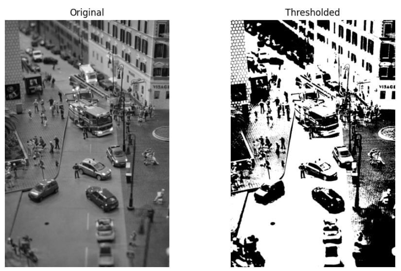
The above thresholded result appears overly high-contrast because a single global threshold is applied across the entire image. Variations in lighting and shadows cause many unrelated regions to collapse into pure black or white, fragmenting fine details and merging large areas.

Clustering-based Segmentation

Clustering-based segmentation treats segmentation as a grouping problem. Pixels are grouped based on similarity, usually using color or intensity values. Unlike thresholding, clustering can split an image into multiple regions without predefined rules.

K-means is one of the most common clustering methods used for this purpose.

import cv2
import numpy as np
import matplotlib.pyplot as plt

image = cv2.imread("/content/miniature-4308104_1280.jpg")
image_rgb = cv2.cvtColor(image, cv2.COLOR_BGR2RGB)

pixels = image_rgb.reshape((-1, 3)).astype(np.float32)

K = 3
criteria = (cv2.TERM_CRITERIA_EPS + cv2.TERM_CRITERIA_MAX_ITER, 10, 1.0)

_, labels, centers = cv2.kmeans(
    pixels,
    K,
    None,
    criteria,
    10,
    cv2.KMEANS_RANDOM_CENTERS
)

segmented = centers[labels.flatten()]
segmented_image = segmented.reshape(image_rgb.shape).astype(np.uint8)

plt.figure(figsize=(10, 6))

plt.subplot(1, 2, 1)
plt.title("Original")
plt.imshow(image_rgb)
plt.axis("off")

plt.subplot(1, 2, 2)
plt.title("K-means Segmentation")
plt.imshow(segmented_image)
plt.axis("off")

plt.show()

Output:

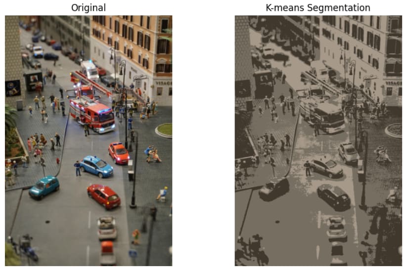
In the above output, the K-means output looks flat and posterized because pixels are grouped only by color similarity, not by spatial location. Objects with similar colors but different meanings end up in the same cluster, while boundaries between real-world objects are not preserved.

Region growing and connected components

Region-based segmentation methods focus on spatial connectivity. Instead of grouping pixels globally, they identify connected regions that share similar properties. This approach is often applied after thresholding to separate individual objects.

import matplotlib.pyplot as plt
from skimage import measure, morphology

labels = measure.label(binary, connectivity=1)
labels_clean = morphology.remove_small_objects(labels, min_size=500)

plt.figure(figsize=(10, 6))

plt.subplot(1, 2, 1)
plt.title("Binary Input")
plt.imshow(binary, cmap="gray")
plt.axis("off")

plt.subplot(1, 2, 2)
plt.title("Connected Components")
plt.imshow(labels_clean, cmap="nipy_spectral")
plt.axis("off")

plt.show()

Output:

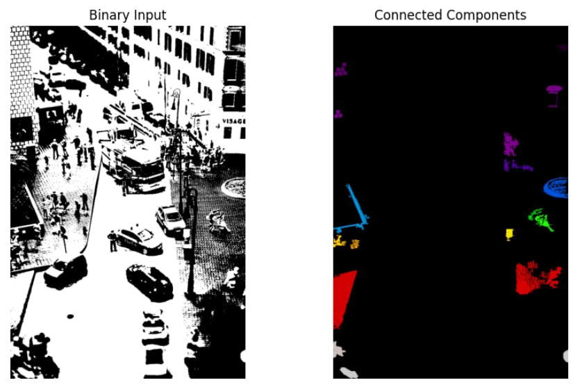
Only a few colored regions remain in the above output because connected component labeling keeps only spatially connected areas that meet the size threshold. Smaller regions and noise are removed, leaving isolated blobs rather than a whole scene segmentation.

Pros & Cons

Thresholding, clustering, and region-based methods are fast, easy to implement, and require no training data. They are highly interpretable, making it clear why a pixel or region was assigned to a segment. In controlled environments with stable lighting and simple backgrounds, these techniques can be surprisingly effective and are often used as preprocessing steps in larger image processing pipelines.

However, these methods rely on strong assumptions about the input image. Thresholding struggles with uneven illumination, clustering ignores spatial structure, and region growing depends heavily on clean binary masks. As scene complexity increases, manual tuning becomes unavoidable, and results fail to generalize across different images.

These limitations are the main reason modern segmentation workflows increasingly rely on learned, data-driven models, which we will explore in the following sections.

Classic Segmentation Pipelines with scikit-image and OpenCV

Classic image segmentation is usually implemented as a step-by-step pipeline, where each stage improves the quality of the next. Instead of relying on a single algorithm, these pipelines combine simple, interpretable operations that work well in controlled settings.

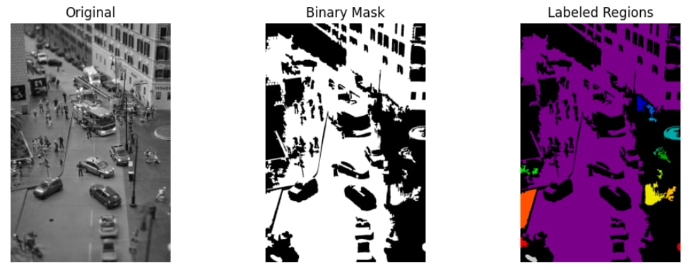
Step 1: Preprocessing

The pipeline starts by preparing the image for segmentation. This typically includes converting to grayscale or another color space and applying smoothing to reduce noise and lighting variations that can break thresholding or clustering.

Step 2: Segmentation

Next, a rule-based method, such as global or adaptive thresholding, color clustering, or edge detection, is applied. This step produces a binary mask or a coarse segmentation that separates regions of interest from the background.

Step 3: Post-processing and region analysis

Finally, morphological operations clean up the segmentation by removing minor artifacts, filling holes, and separating touching regions. Connected component labeling or contour detection is then used to identify individual regions and extract beneficial properties.

Here’s an example with scikit-image:

import matplotlib.pyplot as plt
from skimage import io, filters, morphology, measure

# Step 1: Load and preprocess
image = io.imread("/content/miniature-4308104_1280.jpg", as_gray=True)
smoothed = filters.gaussian(image, sigma=1.0)

# Step 2: Segment
threshold = filters.threshold_otsu(smoothed)
binary = smoothed > threshold

# Step 3: Post-process and label
cleaned = morphology.remove_small_objects(binary, min_size=500)
cleaned = morphology.remove_small_holes(cleaned, area_threshold=500)
labels = measure.label(cleaned)

# Visualize results
plt.figure(figsize=(12, 4))

plt.subplot(1, 3, 1)
plt.title("Original")
plt.imshow(image, cmap="gray")
plt.axis("off")

plt.subplot(1, 3, 2)
plt.title("Binary Mask")
plt.imshow(cleaned, cmap="gray")
plt.axis("off")

plt.subplot(1, 3, 3)
plt.title("Labeled Regions")
plt.imshow(labels, cmap="nipy_spectral")
plt.axis("off")

plt.show()

Output:

And here’s an example with cv2:

import cv2
import numpy as np
import matplotlib.pyplot as plt

# Step 1: Load and preprocess
image = cv2.imread("/content/miniature-4308104_1280.jpg")
gray = cv2.cvtColor(image, cv2.COLOR_BGR2GRAY)
blurred = cv2.GaussianBlur(gray, (5, 5), 0)

# Step 2: Segment
_, binary = cv2.threshold(
    blurred, 0, 255, cv2.THRESH_BINARY + cv2.THRESH_OTSU
)

# Step 3: Post-process and extract regions
kernel = cv2.getStructuringElement(cv2.MORPH_RECT, (3, 3))
cleaned = cv2.morphologyEx(binary, cv2.MORPH_OPEN, kernel)

contours, _ = cv2.findContours(
    cleaned, cv2.RETR_EXTERNAL, cv2.CHAIN_APPROX_SIMPLE
)

# Draw detected regions
output = image.copy()
cv2.drawContours(output, contours, -1, (0, 255, 0), 2)

# Visualize results
plt.figure(figsize=(12, 4))

plt.subplot(1, 3, 1)
plt.title("Original")
plt.imshow(cv2.cvtColor(image, cv2.COLOR_BGR2RGB))
plt.axis("off")

plt.subplot(1, 3, 2)
plt.title("Binary Mask")
plt.imshow(cleaned, cmap="gray")
plt.axis("off")

plt.subplot(1, 3, 3)
plt.title("Detected Regions")
plt.imshow(cv2.cvtColor(output, cv2.COLOR_BGR2RGB))
plt.axis("off")

plt.show()

Output:

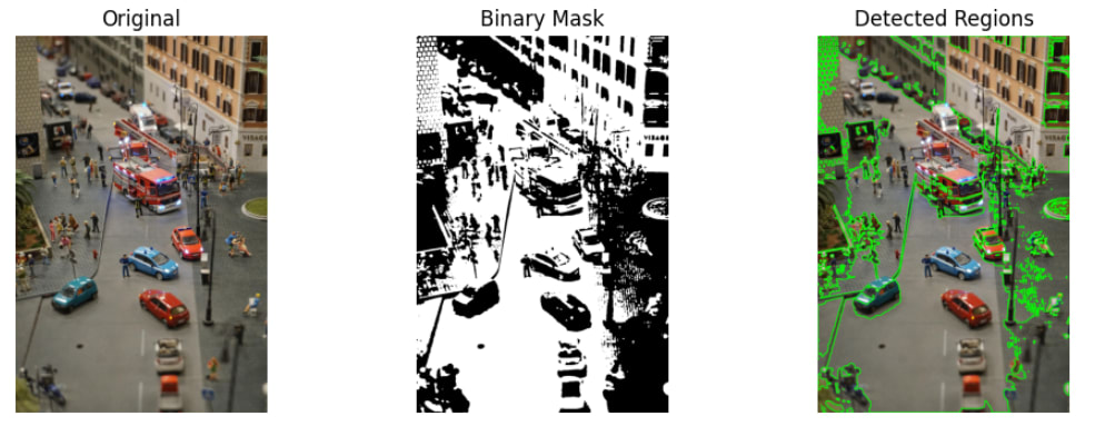
As scenes become more complex, lighting varies, and objects overlap or change appearance, these rule-based pipelines quickly reach their limits. This is where modern deep learning–based segmentation methods become the preferred choice. Instead of relying on fixed rules, these models learn rich representations directly from data, leading to far better accuracy and robustness across diverse images.

Modern Deep Learning Approaches: U-Net, Mask R-CNN, and Transformers

Deep learning has reshaped image segmentation by replacing hand-crafted rules with learned models that understand both local details and global context. Three families of models dominate modern segmentation workflows: U-Net, Mask R-CNN, and transformer-based models.

U-Net for Pixel-level Segmentation

U-Net is a foundational architecture for semantic segmentation, initially designed for biomedical images. It follows an encoder–decoder architecture with skip connections that preserve fine spatial details while capturing broader context. U-Net excels when trained on task-specific datasets that require precise pixel boundaries.

U-Net is not included in core PyTorch, so we install a dedicated library that provides a reference implementation via pip install segmentation-models-pytorch

Let’s check out a U-Net example using an ImageNet-initialized encoder:

import torch
import segmentation_models_pytorch as smp
from torchvision import transforms
from PIL import Image
import matplotlib.pyplot as plt

# Load a pretrained U-Net model
model = smp.Unet(
    encoder_name="resnet50",
    encoder_weights="imagenet",
    in_channels=3,
    classes=1
)
model.eval()

# Load and preprocess image
image = Image.open("/content/miniature-4308104_1280.jpg").convert("RGB")
transform = transforms.Compose([
    transforms.Resize((256, 256)),
    transforms.ToTensor(),
])

input_tensor = transform(image).unsqueeze(0)

# Run inference
with torch.no_grad():
    mask = model(input_tensor)

# Visualize segmentation mask
mask = mask.squeeze().cpu().numpy()

plt.figure(figsize=(6, 4))
plt.title("U-Net Segmentation Mask")
plt.imshow(mask, cmap="gray")
plt.axis("off")
plt.show()

Output:

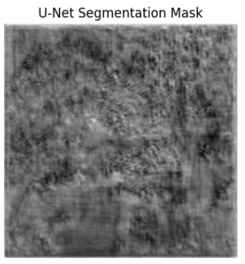
The output appears blurry and unstructured because the U-Net decoder hasn’t been trained for this task. Only the encoder is initialized with ImageNet weights, while the decoder layers are randomly initialized. Without training on labeled segmentation masks, the model produces raw feature activations rather than meaningful object boundaries.

But, this behavior is expected. U-Net is not a plug-and-play segmentation model; it must be trained on task-specific data before producing usable results.

Mask R-CNN for Instance Segmentation

Mask R-CNN performs instance segmentation, meaning it detects individual objects in an image and predicts a separate segmentation mask for each one. Unlike semantic segmentation models, which label every pixel globally, Mask R-CNN distinguishes between multiple instances of the same class, such as different people or vehicles in the same scene.

This makes Mask R-CNN well-suited for tasks like people segmentation, vehicle detection, retail analytics, and robotics, where separating individual objects matters more than labeling the entire background.

The example below uses a pretrained Mask R-CNN model trained on the COCO dataset. It detects objects, draws bounding boxes, overlays segmentation masks, and labels each detected instance.

import torch
import torchvision
import numpy as np
import cv2
import matplotlib.pyplot as plt
from torchvision.transforms import functional as F
from PIL import Image

# COCO class labels
COCO_CLASSES = [
    "__background__", "person", "bicycle", "car", "motorcycle", "airplane", "bus",
    "train", "truck", "boat", "traffic light", "fire hydrant", "stop sign",
    "parking meter", "bench", "bird", "cat", "dog", "horse", "sheep", "cow",
    "elephant", "bear", "zebra", "giraffe", "backpack", "umbrella", "handbag",
    "tie", "suitcase", "frisbee", "skis", "snowboard", "sports ball", "kite",
    "baseball bat", "baseball glove", "skateboard", "surfboard", "tennis racket",
    "bottle", "wine glass", "cup", "fork", "knife", "spoon", "bowl", "banana",
    "apple", "sandwich", "orange", "broccoli", "carrot", "hot dog", "pizza",
    "donut", "cake", "chair", "couch", "potted plant", "bed", "dining table",
    "toilet", "tv", "laptop", "mouse", "remote", "keyboard", "cell phone",
    "microwave", "oven", "toaster", "sink", "refrigerator", "book", "clock",
    "vase", "scissors", "teddy bear", "hair drier", "toothbrush"
]

# Load pretrained Mask R-CNN model
model = torchvision.models.detection.maskrcnn_resnet50_fpn(pretrained=True)
model.eval()

# Load image
image = Image.open("/content/miniature-4308104_1280.jpg").convert("RGB")
image_tensor = F.to_tensor(image)

# Run inference
with torch.no_grad():
    prediction = model([image_tensor])[0]

# Prepare image for drawing
image_np = np.array(image)
output = image_np.copy()

# Confidence threshold
threshold = 0.9

# Label styling
font = cv2.FONT_HERSHEY_SIMPLEX
font_scale = 0.7
font_thickness = 2
padding = 4

for box, label, score, mask in zip(
    prediction["boxes"],
    prediction["labels"],
    prediction["scores"],
    prediction["masks"]
):
    if score < threshold:
        continue

    # Bounding box
    x1, y1, x2, y2 = box.int().tolist()
    cv2.rectangle(output, (x1, y1), (x2, y2), (0, 255, 0), 2)

    # Label text
    class_name = COCO_CLASSES[label]
    label_text = f"{class_name}: {score:.2f}"

    # Text size
    (text_width, text_height), baseline = cv2.getTextSize(
        label_text, font, font_scale, font_thickness
    )

    # Background rectangle
    cv2.rectangle(
        output,
        (x1, y1 - text_height - baseline - padding * 2),
        (x1 + text_width + padding * 2, y1),
        (0, 255, 0),
        -1
    )

    # Text
    cv2.putText(
        output,
        label_text,
        (x1 + padding, y1 - baseline - padding),
        font,
        font_scale,
        (0, 0, 0),
        font_thickness,
        lineType=cv2.LINE_AA
    )

    # Overlay segmentation mask
    mask = mask[0].cpu().numpy()
    output[mask > 0.5] = (
        output[mask > 0.5] * 0.5 + np.array([0, 255, 0]) * 0.5
    )

# Display result
plt.figure(figsize=(8, 6))
plt.imshow(output)
plt.axis("off")
plt.show()

Output:

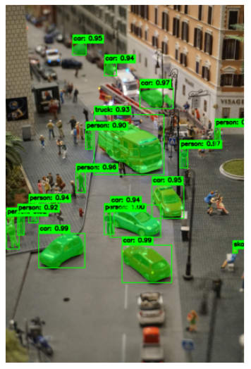
We can see labelled image segments in the above output. Reducing the detection threshold results in more labeled segments in the image. Mask R-CNN works well out of the box because it is pretrained on large, diverse datasets and doesn’t require task-specific retraining for basic object segmentation.

Transformers for Vision Segmentation and Detection

Transformer-based models are commonly used in autonomous driving, robotics, and large-scale visual understanding systems where global context and accuracy are critical. Instead of relying only on local convolutional filters, they model long-range relationships across the entire image. Many modern systems combine transformers with convolutional backbones for improved performance.

Here’s an example that uses a pretrained transformer-based model for image segmentation.

import torch
import cv2
import numpy as np
import matplotlib.pyplot as plt
from transformers import DetrImageProcessor, DetrForObjectDetection
from PIL import Image

# Load image
image = Image.open("/content/miniature-4308104_1280.jpg")

# Load pretrained DETR model
processor = DetrImageProcessor.from_pretrained("facebook/detr-resnet-50")
model = DetrForObjectDetection.from_pretrained("facebook/detr-resnet-50")

# Run inference
inputs = processor(images=image, return_tensors="pt")
outputs = model(**inputs)

target_sizes = torch.tensor([image.size[::-1]])
results = processor.post_process_object_detection(
    outputs, target_sizes=target_sizes, threshold=0.9
)[0]

# Prepare image for drawing
image_cv = cv2.cvtColor(np.array(image), cv2.COLOR_RGB2BGR)

# Label styling (same idea as Mask R-CNN)
font = cv2.FONT_HERSHEY_SIMPLEX
font_scale = 0.7
font_thickness = 2
padding = 4

for score, label, box in zip(
    results["scores"],
    results["labels"],
    results["boxes"]
):
    x1, y1, x2, y2 = box.int().tolist()
    cv2.rectangle(image_cv, (x1, y1), (x2, y2), (0, 255, 0), 2)

    label_text = f"{model.config.id2label[label.item()]}: {score:.2f}"

    # Measure text
    (text_width, text_height), baseline = cv2.getTextSize(
        label_text, font, font_scale, font_thickness
    )

    # Background rectangle
    cv2.rectangle(
        image_cv,
        (x1, y1 - text_height - baseline - padding * 2),
        (x1 + text_width + padding * 2, y1),
        (0, 255, 0),
        -1
    )

    # Draw text
    cv2.putText(
        image_cv,
        label_text,
        (x1 + padding, y1 - baseline - padding),
        font,
        font_scale,
        (0, 0, 0),  # black text for contrast
        font_thickness,
        lineType=cv2.LINE_AA
    )

# Display result
plt.figure(figsize=(8, 6))
plt.imshow(cv2.cvtColor(image_cv, cv2.COLOR_BGR2RGB))
plt.axis("off")
plt.show()

Output:

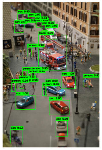
We can see that, with the same threshold of 0.9, the transformer-based ResNET model detects more segments.

Choosing the Right Segmentation Approach

The right image segmentation approach depends on the problem we are solving and the constraints of our data.

Classic techniques (such as thresholding and region-based pipelines) work well when image conditions are stable, backgrounds are simple, and transparency or speed matters more than accuracy. They are perfectly fine for document processing, industrial inspection, and preprocessing tasks.

Deep learning models are better suited for more complex, real-world scenes. U-Net is ideal when we need precise pixel-level masks and have labeled data to train on. Mask R-CNN is the right choice when separating individual object instances matters, while transformer-based models excel in scenes where global context and robustness are critical.

In practice, many production systems combine classic preprocessing with deep learning models to balance performance, accuracy, and cost.

How to Evaluate Segmentation: IoU, Dice, Precision/Recall, and Visual Debugging

Once we generate segmentation outputs, the next critical step is evaluation. Unlike classification, segmentation quality depends on how closely predicted masks align with ground truth at the pixel level. A model can look reasonable visually while still performing poorly quantitatively, which is why standardized evaluation metrics are essential.

• Intersection over Union (IoU): Also known as the Jaccard Index, this measures the overlap between a predicted and a ground-truth mask, and penalizes both false positives and false negatives. It is computed as the area of overlap divided by the area of union between the two masks. Higher IoU values indicate better spatial alignment between predictions and ground truth.
• Dice Coefficient: The Dice coefficient is closely related to IoU but places more emphasis on overlapping regions. It’s commonly used in medical and scientific segmentation tasks, where small structures and class imbalance are frequent. Although Dice scores are typically higher than IoU for the exact prediction, both metrics usually reflect the same overall segmentation quality.
• Precision and Recall for Segmentation: This method can be applied to segmentation by treating each pixel as a classification decision. Precision measures how many predicted foreground pixels are correct, while recall measures how many ground truth foreground pixels are successfully detected. High precision with low recall indicates conservative predictions, while high recall with low precision suggests over-segmentation.

These metrics become especially important when segmentation outputs feed into downstream systems.

But, quantitative metrics alone aren’t usually enough. Visual inspection helps us uncover systematic issues such as boundary errors, merged instances, or noisy predictions that metrics alone may not reveal. Overlaying predicted masks on the original image or comparing predictions side by side with ground truth often explains why a metric is high or low.

In practice, reliable segmentation systems combine numerical evaluation with visual debugging to ensure models are both accurate and dependable in real-world conditions.

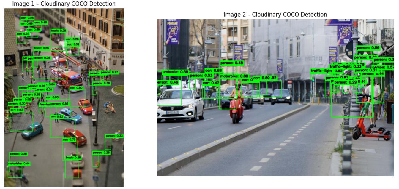
Efficient Image Segmentation with Cloudinary

Cloudinary is a cloud-based media management platform that provides image storage, transformation, optimization, and built-in computer vision capabilities. In addition to handling image delivery and performance, Cloudinary offers pretrained object detection models that can be invoked during image upload without running any local machine learning code.

In the example below, we use Cloudinary’s COCO object detection to analyze two images and draw bounding boxes around detected objects. To follow along, we only need two things: a Cloudinary account and Cloudinary API credentials.

The example uploads each image, retrieves the detection metadata returned by Cloudinary, downloads the processed image, and visualizes the detected objects side by side. This approach allows us to add object detection to an application without managing models, GPUs, or inference pipelines ourselves.

import cloudinary
import cloudinary.uploader
import cloudinary.api

import cv2
import numpy as np
import matplotlib.pyplot as plt
import requests

# --------------------------------------------------
# Configure Cloudinary
# --------------------------------------------------
cloudinary.config(
    cloud_name="YOUR_CLOUD_NAME",
    api_key="YOUR_API_KEY",
    api_secret="YOUR_API_SECRET",
    secure=True,
)

# Images to process
image_paths = [
    "/content/miniature-4308104_1280.jpg",
    "/content/traffic-7296015_1280.jpg",
]

annotated_images = []

for image_path in image_paths:

    # Upload image and run COCO detection
    result = cloudinary.uploader.upload(
        image_path,
        detection="coco",
    )

    detections = (
        result["info"]
        ["detection"]
        ["object_detection"]
        ["data"]
        ["coco"]
        ["tags"]
    )

    # Download image from Cloudinary
    image_url = result["secure_url"]
    image_bytes = requests.get(image_url).content

    image = cv2.imdecode(
        np.frombuffer(image_bytes, np.uint8),
        cv2.IMREAD_COLOR
    )

    output = image.copy()

    # Label styling
    font = cv2.FONT_HERSHEY_SIMPLEX
    font_scale = 0.6
    font_thickness = 2
    padding = 4

    # Draw bounding boxes
    for label, objects in detections.items():
        for obj in objects:
            confidence = obj["confidence"]
            x_center, y_center, w, h = obj["bounding-box"]

            x1 = int(x_center - w / 2)
            y1 = int(y_center - h / 2)
            x2 = int(x_center + w / 2)
            y2 = int(y_center + h / 2)

            cv2.rectangle(output, (x1, y1), (x2, y2), (0, 255, 0), 2)

            label_text = f"{label}: {confidence:.2f}"

            (tw, th), baseline = cv2.getTextSize(
                label_text, font, font_scale, font_thickness
            )

            cv2.rectangle(
                output,
                (x1, y1 - th - baseline - padding * 2),
                (x1 + tw + padding * 2, y1),
                (0, 255, 0),
                -1
            )

            cv2.putText(
                output,
                label_text,
                (x1 + padding, y1 - baseline - padding),
                font,
                font_scale,
                (0, 0, 0),
                font_thickness,
                lineType=cv2.LINE_AA
            )

    annotated_images.append(output)

# --------------------------------------------------
# Display images side by side
# --------------------------------------------------
plt.figure(figsize=(14, 6))

for i, img in enumerate(annotated_images, start=1):
    plt.subplot(1, 2, i)
    plt.title(f"Image {i} - Cloudinary COCO Detection")
    plt.imshow(cv2.cvtColor(img, cv2.COLOR_BGR2RGB))
    plt.axis("off")

plt.tight_layout()
plt.show()

Output:

Frequently Asked Questions

Do we always need deep learning for image segmentation?

No. Classic techniques such as thresholding, connected components, and morphology are often sufficient when image conditions are controlled and predictable. Deep learning becomes necessary when scenes are complex, lighting varies, or objects overlap and change appearance.

Is Cloudinary replacing deep learning frameworks like PyTorch or TensorFlow?

No. Cloudinary complements these frameworks rather than replacing them. It provides ready-to-use computer vision capabilities for everyday tasks like object detection and tagging, while custom or highly specialized segmentation models still benefit from dedicated deep learning frameworks.

When should we choose a cloud-based solution over a self-hosted pipeline?

We typically choose a cloud-based solution when scalability, reliability, and integration speed matter more than complete model control. Cloud services are handy for large-scale image processing, rapid prototyping, and production systems where maintaining infrastructure would add unnecessary complexity.